Among the flurry of deals announced over the past month and a half, a couple raised eyebrows:

• November 19: Oakland Athletics signed free agent DH Billy Butler.
• December 14: Kansas City Royals signed free agent 1B Kendrys Morales.

(That’s how the transactions were listed on mlb.com. I have no idea why Billy Butler, who started 108 games at DH in 2014 and 35 at first base, is listed as a DH, but Kendrys Morales, who started 71 games at DH and 26 at first, is listed as a first baseman.)

The logic behind these signings made sense superficially: The A’s signed Butler, who was the Royals’ DH in 2014, because Oakland DHs hit a middle-infielder-esque .215/.294/.343 last year. The Royals signed Morales to take Butler’s place. What was a little more surprising was the money: three years for $30 million for Butler, two years for $15.5 million plus an $11 million mutual option/$1.5 million buyout in 2017 for Morales.

The reason that’s surprising is that both were below-average hitters in 2014. Butler had a wRC+ of 79 as a DH, while Morales’s was 62. Among the eleven players with at least 200 plate appearances at DH last season, Morales’s wRC+ ranked eleventh and Butler’s ninth.

That’s the thing about designated hitters: They play the ultimate You had one job… position. All they’re supposed to do is hit. There will never be a Derek-versus-Ozzie, bat-versus-glove debate about DHs. They’re all bat. And while wRC+ doesn’t encompass baserunning contributions, DHs are generally plodders like Butler, who went from first to third on a single only once in 31 opportunities last year, so that doesn’t differentiate them. (There have been only 12 seasons in which a player’s gotten more than 15 stolen bases as a DH, and five of those were by one guy, Paul Molitor.)

(Another DH fun fact: The American League adopted the designated hitter after the 1972 season, when the league batted .239/.306/.343, equating to a .297 wOBA. The worst season since then? 2014: .253/.316/.390, .312 wOBA.)

Designated hitters are paid to hit, not to field and run. So why do DHs who are below-average hitters stay on rosters, much less sign multi-year free agent contracts? Before I try to answer that, here’s another tidbit about designated hitters. This is a list of the number of American League players, by position, who qualified for the batting championship last year (i.e., 502 plate appearances):

• Catchers: 1
• First basemen: 4
• Second basemen: 8
• Shortstops: 9
• Third basemen: 7
• Left fielders: 5
• Center fielders: 7
• Right fielders: 5
• Designated hitters: 1

Salvador Perez was the only player to amass 502 plate appearances as a catcher. That’s understandable, given the demands of the position. But why was David Ortiz the only player to get 502 plate appearances as a DH? It’s clearly not the physical strain of being a designated hitter. So let’s lower the bar a bit and count the number of players, by position, to get 400 plate appearances–regulars, if not batting title qualifiers:

• Catchers: 9
• First basemen: 10
• Second baseman: 11
• Shortstops: 11
• Third basemen: 11
• Left fielders: 7
• Center fielders: 10
• Right fielders: 7
• Designate hitters: 4

Yikes. That makes it look even worse. There were fewer regular designated hitters than there were regulars at any other position. Has this always been the case: unremarkable hitters who aren’t even regulars?

To answer this question, the chart below shows, for every season since the advent of the DH in 1973, the percentage of teams with a DH with 502 plate appearances, the percentage with a DH with 400 plate appearances, and the aggregate OPS+ for all DHs. (I chose the percentage of teams, rather than the the number of DHs, to account for the increase in American League teams from 12 in 1973 to 14 in 1976 and 15 in 2013. And I used OPS+ because that’s the only relative  metric I could find with splits data going all the back to 1973.)

As you can see, there were roughly three eras for DHs:

• 1973-1993: Teams trying to figure out how to optimize the position, with playing time and performance fluctuating, including a nadir of a 96 OPS+ in 1985
• 1994-2007: Slightly fewer regular DHs but the position generating the most offense in its 42-year history
• 2008-2014: Reduced offense and sharply fewer full-time DHs

Let’s examine those three eras in detail. When the DH was first implemented, American League teams relied heavily on aging sluggers. From 1973 to 1976, the DHs with the most plate appearances were Tommy Davis (in his age 34-37 seasons), Tony Oliva (34-37), Frank Robinson (37-40), Deron Johnson (34-37), Willie Horton (30-33), and Rico Carty (33-36).

This began to shift with Hal McRae, whom the Royals acquired via a trade with the Reds at the end of the 1972 season, when he was 27. He started 134 games at DH in 1973-75, and was a full-time DH for the remainder of his career. He received MVP votes in four seasons. In 1978, 29-year-old Angel Don Baylor finished seventh in the MVP vote, primarily as a DH (102 starts at DH, 56 in the field) and he won the MVP the next year starting 97 games in the outfield and 65 at DH. There were still plenty of old DHs by the late 1970s — Horton was 36 in 1979 when he became one of only two DHs in history to play 162 games at the position — but it wasn’t the exclusive province of old guys.

Still, there were variations in play. The year 1980 is the only non-strike-shortened season in which no DH qualified for the batting title, and that was largely because of a changing of the guard: Carty retired, Lee May and Mitchell Page neared the end of their careers, Horton played his last season, and Rusty Staub inexplicably got 40% of his plate appearances as a 1B/OF.

As you can see by the chart, the performance of DHs took off after 1993, a year during which four former MVPs and/or future Hall of Famers provided 400+ plate appearances of subpar performance as a DH: George Brett (.265/.311/.431, 95 OPS+), Andre Dawson (.266/.308/.432, 94 OPS+), Dave Winfield (.258/.313/.406, 90 OPS+), and George Bell (.217/.243/.363, 59 OPS+). Brett, 40, and Bell, 33, were in their last seasons, while Winfield, 41, and Dawson, 38, were in their last years as regulars.

That led to another changing of the guard in 1994, and fourteen straight years in which DH OPS+ was 105 or higher, accounting for half of the 28 such seasons in the DH’s 42-year history. Of the nine seasons during which DHs had a combined OPS+ greater than 110, six occurred during 1994-2007. This was the heyday of Edgar Martinez, the greatest DH, of course, but Ortiz (4), Chili Davis (3), Travis Hafner (3), Frank Thomas (3), Ellis Burks (2),  Jose Canseco (2), Juan Gonzalez (2), and Jim Thome (2) all had multiple seasons with an OPS+ of 125 or more as a regular DH during those years.

(I know what you’re thinking: Hmm, 1994 to 2007: PEDs. Yes, but the statistics I’ve used throughout this analysis — wRC+ and OPS+ — are relative figures. The league average, every year, is 100. When DHs compiled a 114 OPS+ in 1998-99, it meant they were 14% better than the inflated averages of the time, a level never attained before or since. So unless there’s some reason DHs were more chemically enhanced, or benefited more from such enhancement, than other players, it’s not a PED thing. And no, it’s not because of the alleged career-prolonging properties of PEDs, as only five of the 21 seasons of OPS+ over 124 cited above were amassed by players older than 35. Nine of the player-seasons were compiled by hitters in their 20s, and five occurred in 2006 and 2007, after the implementation of MLB’s drug policy.)

That brings us 2008-2014. The average OPS+, which was 104 in the 1973-93 period and 109 during 1994-2007 has receded to 106 over the past seven seasons. More strikingly, while the percentage of teams employing a full-time DH (400+ plate appearances) has declined steadily, from 43% in the first 21 years to 38% in the next 14 to 36% in the past seven, the percentage qualifying for the batting title has nosedived, from 27% over the first 35 years of the DH to 16% in the seven years since. In 2008, Thome was the only player who qualified for the batting title as a DH, as was Butler in 2012 and Ortiz in 2014. Prior to those seasons, the only times that happened were in the nascent DH seasons of 1980 (noted above) and 1976 (Carty).

So what’s happening now, and how might it inform the Butler and Morales contracts? I think that the decline in DH performance relative to the league and the decline of full-time DHs are related, because they both stem from the construction of pitching staffs in general, and the modern bullpen in particular. In 1973, the first year of the DH, teams commonly carried 10-11 pitchers on their 25-man rosters. Now they usually have 12, sometimes as many as 13. That leaves less room for a full-time player who can’t play in the field and more need for positional flexibility. As Dave Cameron wrote nearly five years ago:

Teams are choosing to increase their flexibility, even if it comes at the expense of some production. Increasingly, teams want the option to use the DH spot as a pseudo off day for their regulars, or as a fall back plan if their banged-up position player is unable to acceptably field his position. With the move towards 12 man pitching staffs, limited bench sizes put a premium on roster flexibility, and teams are reacting by devaluing players who can’t play the field.

In 2014, eight players played at least 15 games at DH (the extreme right side of the defensive spectrum) and 15 games at catcher, second base, or shortstop (the extreme left side). Breaking that combination down by the eras I defined above, it works out to:

• 1973-1993: 91 occurrences, or 4.3 players per season
• 1994-2007: 50 occurrences, or 3.6 players per season
• 2008-2014: 42 occurrences, or 6.0 players per season

Positional flexibility allows teams to get maximum utility from scarce roster spots, but it doesn’t boost batting by DHs. The eight players in 2014 who played at least 15 games at second, short, or catcher as well as DH were J.P. Arencibia (64 wRC+), Alberto Callaspo (68 wRC+), Logan Forsythe (80 wRC+), John Jaso (121 wRC+), Derek Jeter (73 wRC+), Josmil Pinto (101 wRC+), Dioner Navarro (98 wRC+), and Sean Rodriguez (99 wRC+): One good hitter, three average hitters, and four lousy ones. That doesn’t help the aggregate numbers for designated hitters. Add to that the “DH Penalty,” i.e. the observation that hitters tend to perform worse at DH than when playing in the field — which Mitchel Lichtman calculates in this article to be about 14 points in wOBA — and we can expect increased positional flexibility to erode the offensive contributions of designated hitters.* Jaso, an extreme example, hit .298/.362/.488 in 50 games as a catcher but only .208/.293/.296 in 35 games as a DH.

The DH will remain an offensive position, obviously. And there are obvious risks in drawing conclusions based on just the past seven seasons of data, which admittedly include three above-average years for DHs in aggregate. But given modern roster construction, it’s hard to see DHs consistently generating an outsized contribution to offense as they did in years past. That doesn’t make the below-average performance of Butler and Morales tolerable, but it does make it less of an outlier than it would’ve been previously.

*Lichtman’s data indicate that position players who sometimes were DHs didn’t suffer a greater DH penalty than players like Ortiz or Butler, who rarely play in the field. But as he stated in the above-cited article,

I expected that the penalty would be greater for position players who occasionally DH’d rather than DH’s who occasionally played in the field. That turned out not to be the case, but given the relatively small sample sizes, the true values could very well be different.

Introduction

A few weeks ago I posted a proposal for a regression analysis for an econometric class I am taking with the promise I would post the full analysis when it is complete. Well, its been completed and here is the full analysis, as promised. Its a lot of words so if you don’t care much for how a Probit model works or how to perform a t-test I will go ahead and tell my findinds now.  I found that the speed of a four-seam fastball does help determine the outcome of the pitch–the faster the pitch the lower quality of contact. I also found that movement of a four-seam fastball is statistically insignificant–a four-seam fastball can have zero movement and the outcome will be the same for that pitch. This could be because a four-seam fastball just doesn’t move that much relative to other pitches, I’m not sure though. Also, the model I created has very low goodness of fit measures, which means speed and movement of a four-seam fastball only play a small part in determining the outcome of the pitch. This makes sense: baseball is a complicated game and a lot of variables go into determining an outcome. Without adding even more words to this post below is the paper, in its entirety.

It could easily be said Major League Baseball is in an arms race. Teams have been putting a greater emphasis on finding and developing pitchers who can throw a baseball faster than their peers. Indeed, the average velocity of a fastball has increased every year from 2004 to 2013, with a slight downtick in 2014. From 1990 to 1999, 37 pitchers threw 25 percent or more of their fastballs at 95 MPH or faster; in 2013, 149 pitchers did so. From 2003 to 2008, seven pitchers threw a fastball 100 MPH or faster 20 or more times in a season; from 2009 to 2013, 38 pitchers did so. Teams are trying to find flame-throwers because they believe the faster a ball travels towards home plate, the harder it is for a hitter to make the type of contact resulting in a hit. On the other hand, other factors not emphasized, such as the amount of movement of a fastball may play a role. When a pitcher throws a fastball, it moves. Just as some pitchers can throw a fastball with more velocity, some pitchers can throw a fastball with more movement than others. The relationship between velocity and contact should be the same for movement—the more movement there is, the harder it is to make good contact.

Due to this assumed relationship between velocity, movement, and outcome, I would like to answer the following questions: is it more difficult to hit a fast-moving four-seam fastball than one moving more slowly? Also, is it more difficult to hit a four-seam fastball the more movement it has? Therefore, my hypothesis is twofold: A fast pitch will be more difficult to hit than a slower moving pitch, and the more movement a pitch has, the harder it will be to hit. If my hypothesis is true, more speed and more movement will make a pitch more difficult to hit. The ball from a specific pitch is difficult to hit if a batter swings his bat and fails to make contact with the ball, or the contact made is poor and results in the batter making a strike, if he swings and misses, or an out, if he puts the ball in play.

The body of this paper is organized into six categories: the economic model, the econometric model, the data, the procedures of estimation and inference, the empirical results, and the conclusion. The economic model section explains the composition of the independent variables, the dependent variables, and the error term. It also explains the assumptions as well as provides a general framework for the type of model required for the estimation. The econometric model lays out the functional form of the economic model by formalizing the variables and creating the equations; it also establishes a method to test the statistical significance of the independent variables. The data section explains how the data was gathered, any issues that had to be resolved, and any hesitations about the quality of the data. The procedures of estimation and inference section describes the tools, software, and the specific models chosen to derive the results, why they were chosen, and the characteristics of the model. The empirical results section reports the means of the independent variables, the discrete profile for the outcomes, the parameter estimates, interval estimates, the value of the test statistics, and the goodness of fit measures; it also puts the parameters into the equations. Finally, the conclusion section analyzes the implications from the empirical results and offers possible explanations for the results.

The Economic Model

Independent Variables

A pitcher can throw many types of pitches. The pitcher can try to deceive the batter by throwing a pitch that has a lot of movement, such as a curveball or slider, or a pitch that is slower than it looks like it will be when it leaves the pitcher’s hand, such as a change-up. But no pitcher tries to deceive a hitter when throwing the four-seam fastball. When a pitcher throws a four-seam fastball he is simply trying to throw it as hard and accurate as he can. And this is what teams are searching for—the maximum velocity of a pitcher’s four-seam fastball and the higher the velocity, the better. Even though a pitcher is not trying to induce movement when he throws a four-seam fastball, the ball still moves either horizontally or vertically, which can affect the outcome of the pitch, just as velocity can. This means there will be two independent variables: velocity, measured in MPH, and total movement, which is horizontal plus vertical movement, measured in inches.

Dependent Variables

The dependent variables will be all of the possible per-pitch outcomes that involve the batter attempting to hit the pitch by swinging his bat; this excludes pitches an umpire calls a strike or a ball. These two outcomes are excluded because the batter did not swing his bat, which means the speed or movement of the pitch having any effect on avoiding contact, or inducing poor contact, cannot be discerned.

In addition, because the outcomes are per-pitch, walks and strikeouts are excluded because those outcomes are already accounted for. More specifically, if the batter walks, then he did not swing at the pitch, and it is therefore excluded. If the batter strikes out by swinging and missing, which is accounted for with the swinging-strike outcome, or by being called out by the umpire, then it is excluded because the batter did not swing his bat.

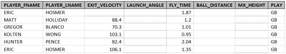
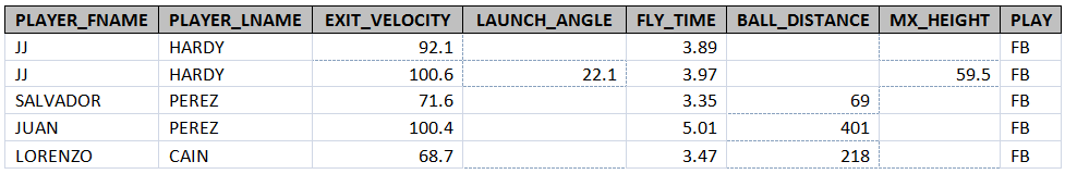
The included outcomes are: swinging strike, foul ball, ground-out, pop-out, fly-out, line-out, single, double, triple, and home run. The difference between a pop-out and a fly-out is who catches the ball: if an infielder catches a ball in the air then it is a pop-out, if an outfielder catches a ball in the air then it is a fly-out. Many types of outs have been included because each type of out can indicate what type of contact was made. For example, if the contact was poor, then the result will either be a ground-out or a pop-out. If the contact was solid, but the batter still made an out, then the result will be a line-out or a fly-out. If the contact did not result in an out, then it will be assumed the contact was good.

From a pitchers perspective the most desirable outcomes are, from most to least desirable: swinging strike, pop-out, ground-out, fly-out, line-out, foul, single, double, triple, and home run. This ranking also reflects a continuous spectrum of contact from softest to hardest. An argument can be made that a swinging strike does not belong on the spectrum because no contact was made. But no contact is still a type of contact; it is the absence of contact, which is the lowest quality of contact and the lowest point on the contact spectrum.

Error Term

The error term will capture the sequencing of the previous pitches, the count, the base-out state, the location of the pitch, and the quality of the defense.

Each pitch will be context neutral; the pitches that preceded it will not be accounted for. This can affect the outcome of the pitch because the absolute speed of the pitch may not matter as much if the previous pitches that a batter has seen in an at bat have been much slower than the four-seam fastball.

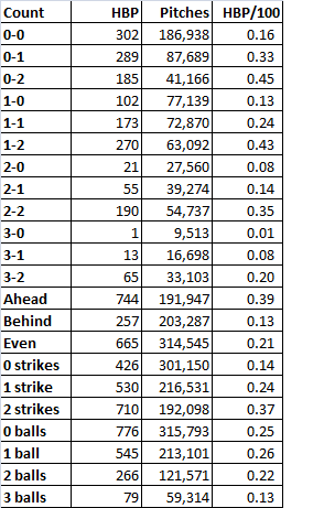
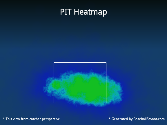
The count of the at bat can affect the outcome of the pitch because batters know, in some counts, pitchers are more likely to throw a four-seam fastball. In this case, the batter may be anticipating the four-seam fastball, which will give the batter an advantage. The base-out state can affect the outcome of the pitch because it can dictate what pitch a pitcher is more likely to throw. The location can also affect the outcome of the pitch because some locations are more difficult for a batter to reach with his bat when he swings. Also, pitchers generally know there are certain locations where most hitters of a certain handedness have difficulty hitting a four-seam fastball if thrown in the particular location, and the location is less sensitive to speed and movement.

The quality of the defense can affect the outcome of the pitch as well because it can turn hits into outs, if the defense is good, or it can turn outs into hits, if the defense is poor. This can cause the ranking of outcomes to be less predictive of the type of contact made for each outcome. For example, a ground ball that gets past an infielder is a single. But the contact made was the type of contact consistent with the contact for a ground-out, not a single. Since a ground-out is ranked third and a single is ranked seventh, the difference in quality of contact between the two outcomes is substantial.

Estimation Methods

Since the dependent variable can take only one of ten possible values the relationship between the independent and dependent variable is not linear and the Ordinary Least Squares model would not be appropriate for our purposes. The best type of model to predict one of the possible outcomes for a pitch given an initial value of velocity and movement is a Limited Dependent Variable model. A Limited Dependent Variable model is used when the value of the dependent variable is restricted to a range of possible outcomes that can be ranked in a meaningful manner. The estimation of the relationship between the independent and dependent variable requires the method to take into account the restriction and ranking. This model was chosen because the range of possible outcomes is restricted and the values are discrete—each pitch can only result in one of ten possible outcomes—and the outcomes are ordered by their value to the pitcher. Also, the relationship between velocity, movement, and the outcome of the pitch requires the ranking of the outcomes to be accounted for because it is assumed velocity and movement influence the type of outcome.

Since the outcomes are also ranked by type of contact, an outcome occurs only if the contact for a particular outcome is greater than the contact required for the outcome located below it and less than the contact required for the outcome located above it. For example, if the contact made was greater than the contact required for a ground-out, but less than the contact required for a line-out, the outcome would most likely be a fly-out.

This type of reasoning implies interval estimates will need to be created for each outcome. Each interval estimate will have a lower limit and an upper limit; if the value the model calculates, given an initial value of velocity and movement, lies between the upper and lower limit, then the outcome the interval estimate represents will be the outcome to most likely occur.

The Econometric Model

Regression Equation   

Formalizing the independent variables, dependent variables, and error term results in the following equations:

O_i= β₁ + β₂*V + β₃*M + ε                           (1)

Where ε ~ (0, σ²)                                         (2)

The right side of equation 1 contains the dependent variable, outcome, and the subscript i represents the type of outcome. The left side of equation 1 has two parts: a structural component and a random component. The structural component contains the independent variables where β₁ is the intercept, β₂ is the estimated coefficient for velocity, V is velocity in MPH, β₃ is the estimated coefficient for movement, and M is horizontal movement plus vertical movement in inches. The random component is the error term, ε; it is the residual that cannot be explained by the variables in the model. The error term is assumed to have a standard normal distribution, which is indicated by equation 2.

Interval Estimates

If equation 1 is less than the lower limit of an outcome ranked two outcomes higher of the upper limit that equation 1 is greater than, the outcome is the one located between these two outcomes. This can be said in terms of quality of contact as well: if the quality of contact a particular amount of velocity and movement is likely to induce is less than the lower limit for the quality of contact required for an outcome located immediately above a particular outcome, but the quality of contact is greater than the upper limit for the quality of contact required for an outcome immediately below a particular outcome, the quality of contact results in the outcome located between the quality of contact required for the upper and lower limit of the particular outcomes. This means equation 1 can be used to create an interval estimate for a particular outcome:

L_Of < β₁ + β₂*V + β₃*M + ε < -L_Oc = O_i                (3)

L_Of is the upper limit for outcome f and -L_Oc is the lower limit for outcome c. Outcome f’s quality of contact is located immediately above the maximum amount of contact required for outcome i and outcome c’s quality of contact is located immediately below the minimum amount of contact required for outcome i. With that being said, interval estimates can be created for all of the outcomes and can be written as:

To make sense of equations 4 through 13, the outcomes have been assigned the following categorical values and subscripts in Table 1: Categorical Values & Subscripts

Using equations 3, and 4 through 12, the interval estimates can be derived for each outcome, those equations are:

L_PO < β₁ + β₂*V + β₃*M + ε = O_SS                             (13)

L_GO < β₁ + β₂*V + β₃*M + ε < -L_SS = O_PO             (14)

L_FO < β₁ + β₂*V + β₃*M + ε < -L_PO = O_GO             (15)

L_LO < β₁ + β₂*V + β₃*M + ε < -L_GO = O_FO             (16)

L_FL < β₁ + β₂*V + β₃*M + ε < -L_FO = O_LO              (17)

L_SG < β₁ + β₂*V + β₃*M + ε < -L_LO = O_FL             (18)

L_DB < β₁ + β₂*V + β₃*M + ε < -L_FO = O_SG             (19)

L_TP < β₁ + β₂*V + β₃*M + ε < -L_SG = O_DB             (20)

L_HR < β₁ + β₂*V + β₃*M + ε < -L_DB = O_TP             (21)

-L_TP > β₁ + β₂*V + β₃*M + ε= O_HR                           (22)

  Hypothesis Testing

Once the estimates for the coefficients are reported, their level of significance can be tested. To do this a null and alternative hypothesis was created:

H_o: β₂ = 0, β₃ = 0                      (23)

H₁: β₂ ≠ 0, β₃≠ 0                        (24)

Equation 23 is the null hypothesis and it states the coefficients for velocity and movement equal 0. This means if one of the coefficients is 0, the predicted outcome and quality of contact will not change. Equation 24 is the alternative hypothesis and it states the coefficients for velocity and movement is not equal to 0. This means the coefficients do influence the outcome and quality of contact. The next step in hypothesis testing is calculating a test statistic. Since the assumption is the error terms have a standard normal distribution and they are homoscedastic—all of the error terms have the same variance—the t-test will be used for the test statistic. The next step is to establish a rejection region. Because the alternative hypothesis is “not equal to” then a two-tail test needs to be used. This is done with the following equation:

t_{(α/2, N-3)} < t < t_{(1-α/2, N-3)}                           (25)

Where α is the critical value for the level of significance, N is the amount of observations, and N-3 is the degrees of freedom—3 is being subtracted because 3 degrees have been used by the coefficients and intercept. The rejection region has two regions: one located in the lower tail of the curve, the other located in the upper tail of the curve. The space to the left of t_(α/2,N-3) is the lower tail and the space to the right of t_{(1-α/2, N-3)} is the upper tail. Equation 25 states the null hypothesis can be rejected for two reasons: if t is greater than t_{(α/2, N-3),} or if it t is less than t_{(1-α, N-3)}. If either of these is true, the null hypothesis is located beyond the critical value somewhere in one of the rejection regions, which means the null hypothesis can be rejected and the alternative hypothesis can be accepted. But, if both of the reasons needed to reject the null hypothesis are false, the null hypothesis is located before the critical value of both tails somewhere in the acceptance region, which means it cannot be rejected and the coefficient being tested could be 0—which is statistically insignificant.

Data

The data was collected from www.BaseballSavant.com. This website maintains the PITCH f/x database, which contains data on every pitch thrown from the 2008 to 2014 season, using high speed cameras located in every Major League ballpark. Since the data from 2008 to 2009 has some classification issues, those years are excluded from the data sets; thus the data sets are from seasons 2010 to 2014. Each data set has approximately 21,000 observations. Since there are five data sets, the total amount of observations is approximately 105,000.

The website allows for many types of filters to be used when searching for data, but the filters used for our purposes are pitch type, pitch result, batted ball result, and at-bat result. The filters for pitch result do not include the type of outcome resulting from the ball being put in play. To get those results the filters for at-bat result had to be used. This resulted in the inclusion of data that was supposed to be excluded. For example, if a four-seam fastball was thrown during an at-bat, but the batter did not swing, then it needs to be excluded, but if the at-bat ended with one of the selected at-bat filters then it was included in the data set. All lines of data containing this type of issue had to be removed from the data sets.

Also, the data on movement came in two components—horizontal movement and vertical movement. Some of the values for horizontal and vertical movement were negative and some were positive. Horizontal movement is positive if the pitch moves towards the right side of home plate, and negative if the pitch moves towards the left side of home plate from the catchers’ perspective. Vertical movement is positive if the pitch drops less than it would from gravity alone, and negative if the pitch drops more than it would from gravity alone. If a pitch had one type of movement that was positive and another type of movement that was negative, the two values would subtract from each other when adding them together and not properly reflect total movement. To prevent this from occurring, the absolute value was taken for each type of movement and then added together.

Since a Limited Dependent Variable model is being used, a new variable had to be created. This variable captures the ranking of each outcome by assigning a numerical value to each type of outcome. Since each outcome was ranked from least to most desirable from the perspective of the pitcher, the least desirable outcome, a home run, was assigned the value of one, and the most desirable outcome, a swinging strike, was assigned the value of ten. Also, a variable had to be created indicating the year from which the data originated. Since there are five years’ worth of data, the variable could take on one of five possible values—1 through 5. This was done because all of the data was combined when put into the program. Having a variable indicating year allowed for a dummy variable to be created in the program so different data sets could be created and regressions could be run on each data set, and then all the data sets combined.

Procedures of Estimation and Inference

The program used to run the regression was SAS, version 9.3. The procedure used to estimate the mean, standard deviation, and the minimum and maximum values for the independent variables was the MEANS procedure. The procedure used to estimate the intercept, coefficients, and interval estimates was the QLIM procedure. The QLIM procedure is a Limited Dependent Variable model, and can use either the Binary Probit or Logit model, or the Ordinal Probit or Logit model. The Binary Probit or Logit model is used when the dependent variable assumes only one of two values. Since the dependent variable has ten possible values, the Binary model was not appropriate for our purposes. The Ordinal Probit or Logit model allows for a dependent variable to assume more than two values and the values can be ranked in either ascending or descending order, which was most appropriate for our purposes. The difference between the Ordinal Probit and Ordinal Logit model is the Ordinal Logit model assumes the error term has a standard Logistic distribution, and the Ordinal Probit model assumes the error term has a standard Normal distribution. Error terms can be assumed to have a standard normal distribution if the dependent variable is influenced by an unobserved continuous variable and the possibilities for the unobserved continuous variable is infinite, even if the possibilities are bounded between a minimum and maximum value.

The outcome of a pitch can be thought of as a proxy for quality of contact—the softer the contact the better the outcome for the pitcher and vice versa. Even though the model has ten dependent categorical ordinal outcomes—which by definition means it is not continuous—it measures a single variable at a distance, which is quality of contact. Quality of contact can be thought of as being continuous: it is a spectrum of infinite possibilities bounded between two values—no contact and perfect contact. Even though perfect contact is a nebulous concept, it still acts as a boundary that cannot be surpassed. This means quality of contact meets the criteria for having error terms that have a standard normal distribution, which means the Ordinal Probit model is the model most appropriate for our purposes.

The purpose of the Ordinal Probit model is to estimate the probability an observation will fall into one of the categorical outcomes. The central idea behind the Ordinal Probit model is there is an unobserved continuous variable underlying the dependent variable, which influences the ordering of the dependent variable. The unobserved continuous variable is quality of contact, which is assumed to determine the outcome, and it is assumed velocity and movement of a pitch influence quality of contact.

The Ordinal Probit model creates upper and lower threshold values partitioning the continuous variable into a series of regions corresponding to one of the ordinal categories representing one of the regions along the continuous spectrum. These upper and lower thresholds create intervals; each interval corresponds to a range of contact required for a particular type of outcome. Quality of contact lies on a continuous spectrum of no contact to perfect. Each outcome occupies a region along the quality of contact spectrum. Each outcome has two threshold values: if the quality of contact worsens and passes an upper threshold quality of contact value of a particular outcome, the outcome will be the outcome ranked immediately below the outcome whose upper threshold quality of contact value was passed, this is a lower limit. If the quality of contact improves and passes the lower threshold quality of contact value of a particular outcome, the outcome will be the outcome ranked immediately above whose lower threshold quality of contact value was passed, this is an upper limit.

The Ordinal Probit model relaxes the constraint that the effect of the independent variables is constant across different predicted values of the dependent variable. The model assumes an S-shaped curve. In each tail section of the curve the dependent variable responds slowly to changes in the independent variables, and as it moves closer towards the middle of the curve, the dependent variable responds faster. This implies as the probability of a particular outcome occurring approaches .5, changes in velocity and movement cause relatively large changes in the probability of a particular outcome occurring. As the probability of a particular outcome occurring approaches 0 or 1, changes in velocity and movement induces relatively small changes in the probability of the particular outcome occurring.

This cascading effect of outcome-probability has intuition: if the probability of an outcome occurring approaches 0, the probability of the outcomes furthest away—either below its lower limit or above its upper limit depending on the type of contact—must be approaching 1. This means as the probability of a particular outcome decreases by a particular amount, the amount it decreases by is allocated disproportionally between the outcomes in a particular direction in descending order, with the outcome ranked immediately above or immediately below receiving the biggest increase in probability of occurrence, and the outcome furthest away probability of occurrence increasing the least, which is closest to 1. Another way to put it is, as velocity and movement changes, contact moves along its spectrum changing the probability of each of outcome occurring; some probabilities increase and some decrease. If the probability of an outcome decreases, the amount it decreases by increases the probability of the outcome located immediately below or above to increase the most, and the outcome located the furthest away to increase the least, with the probability of all the intermediate outcomes increasing or decreasing disproportionally with their distance from the origin.

For example, a home run and swinging strike are on opposite ends of the contact spectrum. If the probability of a home run occurring approaches 0, and the probability of a swinging strike occurring approaches 1, the amount of velocity and movement—and therefore contact—required for the two outcomes is substantially different because the probability of anything occurring in between must be approaching 0, but not at the rate in which the home run contact is approaching 0. As velocity and movement change towards the amount of velocity and movement required to induce the type contact resulting in a home run, then the probabilities of the outcomes located between swinging strike and home run will increase, with the probability of the outcome located immediately below swinging strike, pop-out, increasing the most, and the outcome located immediately below pop-out, ground-out, increasing the second most, and so on, with the probability of a home run occurring increasing the least. As velocity and movement continue to change and contact moves along its spectrum towards the type of contact required for a home run, the probabilities of each outcome change with the outcomes closest to a swinging strike increasing the most until, eventually, the allocation of probability is reversed and the probability of a home run occurring approaches 1 and the probability of a swinging strike occurring approaches 0.

Empirical Results

Discrete Response Profile & Means            

Table 2 is the discrete response profile for seasons 2010 to 2014. It reports the frequency of each outcome and the percent the frequency represents of all the outcomes.

Table 3 contains the amount of observations for each variable, the mean, standard deviation, and the minimum and maximum values for seasons 2010 to 2014.

Parameter Estimates

Table 4 contains the parameter estimates for data from the 2010 to 2014 seasons. It contains the estimates, standard error, t values, and p values for each of the parameters. The standard error indicates the accuracy of the estimate in representing the population. The t and p values test for statistical significance. They both assume the null hypothesis is true and equal to 0. The t value indicates if the estimate is statistically significant from 0, the larger the t value, the more likely the null hypothesis is wrong and the parameter is statistically significant from 0. The p value indicates the probability the null hypothesis is true and the parameter is not statistically significant from 0. The lower the p value the more likely the null hypothesis is false and the parameter is statistically significant from 0.

           Hypothesis Testing

Since the standard error and t value have been reported, their level of significance can be tested. Using the null and alternative hypothesis from equations 23 and 24 and using a critical value of 5 percent, equation 25 can be written as:

t_{(2.5, 107,877)} < 16.10 < t_{(97.5, 107,877)} = -1.960 < 16.1 < 1.960             (26)

t_{(2.5, 107,877)} < -1.81 < t_{(97.5, 107,877)} = -1.960 < -1.81 < 1.960             (27)

Equation 26 is the test hypothesis for velocity. Since -1.960 is less than 16.1 and 16.1 is greater than 1.960, the null hypothesis for velocity is located to the right of the critical value in the upper tail of the curve somewhere in the rejection region, which means it can be stated with 95% confidence that velocity is statistically significant from 0 and influences the quality of contact and the outcome of the pitch, holding movement constant.

Equation 27 is the test hypothesis for movement. Since -1.960 is less than -1.81, but -1.81 is not greater than 1.960 then the null hypothesis for movement is located to the left of the upper tail’s critical value, which is not beyond the critical value in the rejection region, and means the null hypothesis cannot be rejected. This means it can be stated with 95% confidence that movement is not statistically significant from 0. If movement were 0, the quality of contact and outcome of the pitch would not change, holding velocity constant. This means it can be removed from equations 1, 3, and 13 through 22. Regression Equation Since estimates for the parameters have been calculated and their level of significance has been determined, the values can be plugged into equation 1 to get:

O_i= 2.175107 + .017939*V + ε                      (26)

Movement has been removed because it has no effect on the outcome. Also, the error term remains unknown because its precise value cannot be determined using a Limited Dependent Model. The error term takes on a range of values depending on the value of the independent variables and the value of the upper and lower limit of the outcome.

Interval Estimates

Table 5 contains the interval estimates for seasons 2010 to 2014 for each type of outcome. It gives the lower limit, upper limit, standard error, t value, and p value, and the upper limit minus the lower limit, which gives the size of the interval.

Velocity can be removed from equations 13 through 22 and the values from Tables 4 and 5 can be plugged into the equations to get:

4.811196< 2.175107 + .017939*V + ε = O_SS                                                        (27)

4.664113 < 2.175107 + .017939*V + ε < 4.811196 = O_PO                           (28)

4.304515 < 2.175107 + .017939*V + ε < 4.664113 = O_GO                          (29)

4.043806 < 2.175107 + .017939*V + ε < 4.304515 = O_FO                           (30)

3.975195 < 2.175107 + .017939*V + ε < 4.043806 = O_LO                           (31)

2.506700 < 2.175107 + .017939*V + ε < 3.975195 = O_FL                           (32)

2.175107 < 2.175107 + .017939*V + ε < 2.506700 = O_SG                          (33)

1.798627 < 2.175107 + .017939*V + ε < 2.175107 = O_DB                           (34)

0.900493 < 2.175107 + .017939*V + ε < 1.798627 = O_TP                           (35)

0.900493 > 2.175107 + .017939*V + ε = O_HR                                                    (36)

  Goodness of Fit Measures

Goodness of fit measures describes how well the model fits the observations. The measures typically summarize the discrepancy between observed values and the expected values in the model. Since the linear regression model was not used, the goodness of fit measures is not those that are typically expected such as the coefficient of determination, R². Table 6 contains the reported measures for the data from the 2010-2014 seasons.

The most useful of these measures is McFadden’s LRI because it is analogous to R². It is bounded between 0 and 1 and, in theory, can equal 1, meaning the model is a perfect fit for the data, even though most models that are a good fit fall in the range of .2 to .4 (vii). All of the other measures except for the Likelihood Ration (R) and Upper Bound of R (U) are similar to McFadden’s LRI—they’re an attempt to simulate R².

Conclusion

Since the estimated coefficient for velocity is positive, the greater the amount of velocity the lower the quality of contact, meaning a desirable outcome for the pitcher is likely to occur. This supports the first part of the hypothesis. But the estimate for movement was not significantly different from 0, which does not support the second part of the hypothesis. A pitcher is not trying to induce movement when he throws a four-seam fastball and the movement that does occur is relatively little compared to pitches in which a pitcher is trying to induce movement. Indeed, a four-seam fastball rotates backwards, which keeps the ball straight and limits the movement. This relatively small amount of movement may not do much to deceive a hitter and cause him to either swing and miss or make poor contact. It would be interesting to see if the amount of movement in pitches in which a pitcher is trying to induce movement leads to lower quality of contact.

According to Table 2, it appears to be difficult for a pitcher to get a hitter to swing and miss at a four-seam fastball. Hitters make contact 84.35 percent of the time, and swing and miss 15.65 percent of the time. It also appears to be difficult for a hitter to make the type of contact required to not make an out—only 9.8 percent of the outcomes resulted in a hit. When a hitter does make an out the type of contact is mostly poor—54.97 percent of the outs are ground-outs and pop-outs. The outs requiring a bit more solid contact—line-out and fly-out—make up 45.03 percent of all the outs. It also appears the most frequent outcome is a foul. Fouls can be good for a pitcher if they result in strikes, but a foul will only result in a strike if the count has less than two strikes. If the count for the hitter has two strikes, it is good for the hitter because he gets to see another pitch.

Since the interval for the foul is the largest and the intercept is the lower limit for the outcome immediately above it—the single—it is easy to see the model predicts the most likely outcome to be a foul. This makes sense because it was the outcome that occurred most often by a wide margin. But given the ambiguity of the foul in terms of value to the pitcher and hitter, and the quality of contact required to cause a foul, any type of positive analysis will be ambiguous. A statement cannot be made about the value of this outcome except the value changes from the pitcher to the hitter depending on the count.

Since the goodness of fit measure is rather low, the model is not a good fit for the data. This result does not mean the model is not predictive. Rather, it means there are other variables influencing the quality of contact and the outcome of the pitch that are not included in the model. In some ways, this makes sense: baseball is a complicated game and the outcome of a four-seam fastball depends on much more than just velocity and movement. Things such as the location of the pitch, the sequencing of the previous pitches, the handedness of the pitcher and batter, the base/out state, and the count play a large part in determining the outcome of the pitch. If some of these variables were included in the model then its predictive power and goodness of fit would have most likely increased.

Taking the average fastball velocity from table 3, 91.96 MPH, plugging it into equation 26 and ignoring the error term, the value is 3.82, which falls in the interval for foul, as expected. But, in order for the speed to result in a swinging strike, it needs to travel around 147 MPH, or 19 standard deviations above the mean. This doesn’t fit very well with reality—no pitcher will ever throw a pitch at 147 MPH and plenty of hitters swing and miss four-seam fastballs with velocity around the mean. If velocity were the only thing determining the outcome, it would require 147 MPH to result in a swing and miss. But velocity is not the only determinant; it has only a small influence over the outcome of the pitch. This supports the conclusion the model does not fit the data very well and the error term is probably rather large relative to the estimated coefficient for velocity.

In the extremely competitive environment of major league baseball where teams flesh out the smallest advantage to give them an edge over their competitors, it makes sense for them to put a greater emphasis on velocity. It does have an influence on generating favorable outcomes for the pitcher. Therefore the trend in baseball is likely to continue and velocity is going to continue to increase.

Ever since I became enamored by the baseball statistical community, I’ve tried to gather as much information as I could. I registered on several websites dedicated to the analysis of baseball statistics such as baseballprospectus.com or FanGraphs.com or HardballTimes.com. I read every book, article I could get my hands on and even tried my hand at producing my own research and analysis in order to achieve two goals in my life: 1. Publish my research and become a savvy baseball analytical mind; and 2. Work within a baseball organization.

My first basic analysis came in the form of three year projections in order to try my hand at fantasy baseball. Personally, I’m proud to say that my first dip within the analytical waters where fruitful as my projections helped me win my league 3 times out of 5 attempts[1]. But, after many years keeping my projections and questions to myself; I’ve finally felt compelled to start more serious research and publish my questions and results online to share with people interested in these topics. So, without further ado, I give you my first serious publication.

***

Many readers will often find that writers, commentators and analysts highly value a player before they reach their age 30 season. But, once they pass this mark, players will begin to gradually decline; their production will falter, they’re prone to getting injured more than once within the same season, their speed will begin to abandon them. In other words, the shine begins to disappear and is replaced by a shelled version of a player we, the fans, and managers value. Furthermore, I’ve often read in many articles that players even peak at the age of 27 – this being the season where a player will give his (all-time) best performance before beginning that slow decline into retirement.

Now, I have two problems with this:

1. What stats determine that a player’s best season is his age 27 season?
2. Does this peak age season vary for every position or are all players subjected to the same aging curve?

To answer the first question, I used player statistics starting from 1960 up to 2013 and looked specifically at power numbers – slugging percentage, isolated power and on-base plus slugging[2]. I then calculated each player’s age in accordance with their birthday and how old they would be by June 30^th and took this to be their age-season. Once I had this, I began running histograms in order to determine the lowest performance, highest performance, mean and first and third percentiles.

For this analysis, I only used the data for players who were between 20 and 35 years of aged during any given season. What I found, starting with SLG, was that players – power-wise – don’t reach their peak at 27 but after their 30s. A player’s SLG increases gradually as he gets older until he reaches his age 31-32 season. A player will have a mean SLG of 0.437 by age 27, while, during his age-32 season, the mean SLG will be 0.447 – ten percentile points higher or an increase of 2.3%.

So, as we can see, SLG-wise, a player will show a better performance past his 30^th birthday. But maybe I am biased. Maybe if I checked ISO, we will find different results.

What I found were very similar results. A player’s isolated power, again, on the mean, didn’t peak at age 27. The ISO was 0.159. And, the ISO didn’t peak during the age-32 season but a year earlier during the age 31 season. During this season, ISO was 0.167 while the next season it began to decline at 0.165. ISO increases by 5.0% during those five years.

Finally, I decided to take a look at OPS to see if I could find a similar pattern. Again, players mean OPS peaks during their age 32 season, going from 0.784 at their age 27 season to 0.801 by the time they’re 32. It’s not much of an increase (2.2%) but it’s something.

What I can determine, then, is that a player’s power begins to develop once he hits 27 years of age and will gradually increase right up to when he turns 32. But, after this, his power performance will begin to decline, though not by much.

Another thing that I concluded from looking at these three histograms is that, even though there are gradual increases every season.  Player performance – power-wise – will be fairly consistent from one season to the next. Save for the early seasons (21-25 when a player is still developing), there are no surprising jumps in power[3] from one age to the next. Therefore, though we might prefer younger players for cost control reasons, when we need power production, we can’t fully disregard an older player’s power performance. Chances are they will still produce the same.

***

Having checked how power changes as a player ages, I come to my second question: Does the aging curve differ across positions? Well in football – or soccer for Americans – we have four major positions: striker, midfielder, defense and goalkeeper. Through statistical analysis by Arsenal F.C.’s data department, Arsene Wenger, Arsenal’s manager, found that a players decline varies on the position he plays on the field. That is to say, a striker will age differently than a goalkeeper, and a defender will age different to these two positions.

And, as we all know, work at different positions takes a different toll on a player’s body. Catchers will suffer become more fatigued as a season rolls by than players at any other position; shortstops, as well, have a more demanding position that will require more physical effort. We expect different results from each of the three outfield positions. So, it would be natural that players at different positions age differently on the power curve[4].

What I found out was that my thoughts were correct: positioning on the diamond does affect a player’s power performance but not by much. These are the results based on the mean:

As we can see from the data, first basemen will usually be the first position players to peak. After them, the three outfield positions will peak at age 32. Catchers will then follow suit. Finally, the hot corner will peak at 34 and the middle infield will produce more power by the time they turn 35 than any of their previous years.

What we can conclude from this table is the following; because the demand on power from first base more than defense, players will tend to flex their muscles more often than not; whilst primarily defensive positions such as catcher, second base and shortstop will develop more power later in their careers than when they start off. Outfielders, on the other hand, tend to produce power throughout their careers.

The position that does surprise me is the hot corner. I would have expected third basemen to peak earlier in their careers because most players at the position are power hitters. Then again, there are many good defensive third basemen who aren’t big power players (I’m looking at you Juan Uribe).

***

After reviewing all the numbers, I can safely conclude that as players age, power doesn’t decline. On the contrary, power also increases though not by very much. Furthermore, the gradual increase in power at the plate will vary by position, much like a football – soccer – player’s performance will vary according to his position. Therefore, though we may like young players because of their hustle, cost-control and their energy, it doesn’t hurt to carry a few veterans in the lineup, if not to mentor the young ones, to provide some pop within the lineup.

[1] A small sample size, I admit, but nevertheless, a positive achievement as it encouraged me to delve deeper into baseball analytics.

[2] I didn’t look at OBP as I believe that this stat has more to do with a player’s ability at identifying pitch types, though in retrospect, this can also become better as a player ages and gains more experience.

[3] Though there are many outliers as you can see.

[4] I have charts and charts of histograms for each position measuring SLG, ISO and OPS but since I don’t want to oversaturate with information.

FanGraphs Wins Above Replacement is considered by many in the sabermetric community be the holy grail of WAR.  And, even though I’m writing a piece that is critical of fWAR, FanGraphs is still the first website I go to when I want to get a basic understanding of a specific player or team’s value.  Don’t view this article as an attack on fWAR or FanGraphs, both of which I use frequently; instead, consider this article as constructive criticism.

fWAR, specifically for pitchers, is riddled with minor problems that together make the metric less valuable.  In Part 1 of the series, we’re going to look at a hotly debated issue regarding fWAR that has been brought up by other readers before: the fWAR park factors.

According to the FanGraphs glossary, a basic runs park factor is used when calculating fWAR.  Because FIP models ERA, using runs park factors for FIP shouldn’t be a problem.

Unfortunately, this idea simply isn’t true.  The inputs of FIP, HR/9, BB/9, and K/9, only include about 30% of plate appearances.  Some ballparks (Citi Field for example), inflate HR/9 and FIP despite suppressing runs in general.  If Pitcher fWAR is based on FIP, FIP park factors, not runs park factors, must be used.  Below is a table comparing runs and FIP park factors for different teams/ballparks, with FIP park factor equaling ((13*HRPF)+(3*BBPF)-(2*SOPF))/(14), with all of the data coming from the FanGraphs park factors.

In addition, the standard difference between the Basic and FIP park factors was a staggering 5.5.  Clearly, using runs park factors on FIP significantly benefits and hurts certain teams’ Pitcher fWAR.

While the Marlins, Red Sox, Pirates, Twins, and Royals benefit from park factors that overestimate their ballpark’s FIP-inflating ability, the Reds, Brewers, White Sox, Yankees and Mets experience the opposite effect, falsely increasing/decreasing these teams’  Pitcher fWAR.

Looking at the team pitching leaderboards, the effect of this mistake is pronounced on several teams’ fWAR.  For example, the Mets, despite ranking 9th in the National League in FIP while playing in a ballpark that inflates FIP by 2%, rank dead last in the National League in Pitcher fWAR.  Similarly, the Red Sox rank 5th in the AL in Pitcher fWAR despite ranking 10th in the AL in FIP and playing in a ballpark that suppresses FIP by 4%.

Using FIP park factors instead of runs park factors is a simple change that would vastly improve the accuracy of Pitcher fWAR.  In the next segment of “Trying to Improve fWAR”, I’ll examine the league adjustments (or lack thereof) in both Position Player and Pitcher fWAR.

Last time, we analyzed Yu Darvish’s sliders in terms of when they projected as strikes and how pitch movement affected perception, leading batters to swing at pitches outside of the strike zone in the direction of the pitch movement. This time, we will turn our focus to four-seam fastballs. As before, we are using the 2013 data set since the algorithms for this were run before the completion of the 2014 season. To start, we can examine a four-seam fastball from Yu Darvish, his second-most thrown type of pitch in 2013, via simulation using the nine-parameter PITCHf/x data for its trajectory. The chosen fastball from Darvish was thrown roughly down the middle of the strike zone and we also track the projection of the pitch as it approaches the plate.

Note that the pitch, in this case, is simulated at one-quarter actual speed. The strike zone shown is the standard width of the plate and 1.5 to 3.5 feet vertically. The red circle represents the projection of the pitch after removing the remaining PITCHf/x definition of movement from its current location (Note that while the simulation shown above is a GIF, the actual simulation is an interactive PDF where the controls at the bottom of the image can play, rewind,  slow down, etc. the simulation. This is discussed at the end of the article for the interested reader, including a link to several interactive PDFs as well as a tutorial for the controls and the source code written in TeX). Here, the movement causes the pitch to rise, giving the pitch in the simulation a “floating” quality as it never seems to drop.

As in the previous work on sliders, we will start by splitting the four-seamers into four groups based on the pitch location and the batter’s response: strikes (pitches with a 50% chance or better of being called a strike) and balls (lower than 50% chance of being called a strike), and swings and pitches taken. Working with the projections to the front of the plate after removing the remaining movement on the pitch, we can examine how attractive (in terms of probability that the projection will be called a strike) pitches in each of these four categories, on average, are to batters incrementally as they approach the plate.

To begin, for left-handed batters versus Darvish in 2013:

For both types of pitches in the strike zone (red=taken, green=swung at), the average probability of the pitch being called a strike levels off around 20 feet, with strikes swung at peaking at probability 0.919 at 9.917 feet from home plate, then dropping to 0.917 at the plate. Strikes taken reach their maximum at the front of the plate with probability 0.869. The four-seamers swung at outside of the strike zone (blue) average around 0.5 probability of being called a strike up until around 30 feet, before dropping off. The fastballs taken outside the zone (orange) tend to project as low-probability strikes initially and remain so to the front of the plate.

We can simplify this graph to include only swings and pitches taken.

Once again, pitches swung at project as better pitches throughout than those taken. The peak for swings is at 14.083 feet with probability 0.782, and finishes at 0.777. The pitches taken keep increasing in attractiveness all the way to the front of the plate, reaching a called-strike probability of 0.332.

To further examine what is happening in these graphs, we can view the location of these projections from 50 feet to the front of home plate. The color scheme is the same as the four-curve plot above.

Focusing on the blue projections for the moment (swings outside the strike zone), the projections down and to the right of the zone are carried by movement toward the strike zone and most end up as borderline strikes. Those up and to the left project further and further outside the strike zone as they approach the plate, since their direction of movement is roughly perpendicular to the strike zone contour. To get a better idea of the number of each of the four cases in nine regions in and around the strike zone, we can fade the data into the background and replace it in each region by an arrow indicating the direction that the average projection for that area is moving and the number of pitches of that case located there.

Focusing first on the pitches in the strike zone, there is a dearth of projections in the upper-right area, which would be on the inside half of the plate to LHB. The pitches taken in the strike zone tend to skew slightly down and to the left, relative to those swung at. Note that in many of the regions around the strike zone, the samples are quite small so it may be difficult to draw any strong conclusions. With this in mind, these results can be summarized in the following table where the center cell represents the swing percentage in the strike zone and all other cells contain the percentage of swings in that region.

The region with the highest swing percentage is the strike zone, at 59%. The region with the next highest percentage is above the strike zone, which is in the general direction of movement, but here there are only nine data points to rely on for this percentage. It would seem that the regions that induce swings are those where the pitches project in the strike zone and are carried out by movement (above and above-and-left of the zone) and where the pitches project as balls but movement is carrying them toward the zone (below and below-and-right of the zone). Notice that the area below and left of the strike zone has 47 pitches thrown there and only 2 swings, which is where the movement parallels the strike zone.

It would appear, based on these observations, that the location of the pitch, relative to the direction of the movement, has an influence on generating swings outside the strike zone. As with the sliders in the previous article, we will use, as a measure of if the pitch is thrown outside in the direction of movement, the angle between the movement of the four-seam fastballs at 40 feet (the pfx_x and pfx_z variables in the PITCHf/x data set) outside the zone and a vector perpendicular to the strike zone extending to the final location of the pitch at the front of home plate. An angle of zero indicates that the movement of the pitch carried it perpendicularly away from the strike zone. Ninety degrees means that the pitch projection parallels the strike zone due to movement. A one-eighty degree angle means that the pitch is being carried by movement perpendicularly toward the strike zone. Further explanation, including a visual depiction, can be found in the link to the previous article at the top of this page.

To begin, we will look at the distribution of angle versus distance from the strike zone for all of Darvish’s four-seamers outside the zone to lefties.

The distribution, in this case, seems slightly skewed toward having pitches thrown in the general direction of movement. This visual assessment is supported by the percentages in the table (sorted by angle and average distance from the strike zone contour in feet. e.g., 0.5 = 6 inches, 0.33 = 4 inches), with nearly 29% of pitches having an angle of less than 45 degrees and over 58% with an angle less than 90 degrees. The distribution does not seem to have definitive shape.

For all MLB right-handed pitchers in 2013, including Darvish, the distribution is much more clear. There is a swell of pitches thrown with angle between 0 and 90 degrees and within six inches of the strike zone, with 37.5% thrown with an angle of less than 45 degrees, and 61.9% with an acute angle. In conjunction, as the angle increases, the average distance from the strike zone decreases. To get a better handle on the ramifications of this choice of pitch locations, we can further sort the data into swings and pitches taken.

For Darvish, nearly 44% of the pitches swung at had an angle between the vector perpendicular to the strike zone and the movement vector of less than 45 degrees. For those less than 90 degrees, this percentage jumps to nearly 70%. In addition, the average distance outside with angle less than 45% is an average of 4 inches outside whereas, overall, the average is about 3 inches in all directions. We can compare this to Darvish’s right-handed colleagues in 2013:

For MLB righties, the largest area of swings is right around a 30-degree angle. Close to half of the swings, 46.9% to be exact, occur when the angle is less than 45 degree and over two-thirds are for pitches in the general direction of movement. The average distance on four-seamers swung at outside is close to Darvish’s overall, but is almost an inch further out for Darvish for 45-degree or less angles. So for RHP to LHB, pitches thrown in the neighborhood of 30 degrees and within a half-foot of the strike zone tend to induce swings, which is also seen for Darvish. We can now look at the complement of this, pitches taken outside, to see how this distribution compares to swings.

The distribution for Darvish on pitches taken has some semblance to that for all pitches, but the percentages have dropped in all cases. In addition, the average distances across the board are over six inches outside.

For all MLB RHP in 2013, the pitches taken by LHB outside the strike zone are largely located below 90 degrees, with a large number near 60 degrees. Compared to the case of all pitches outside the strike zone, the percentages are not all that dissimilar, but the distances are slightly larger. Putting the two hexplots together to see how they form the plot for all outside pitches, we see that what appears to be one large grouping of data below 90 degrees for all pitches separates into two smaller groupings: one around 30 degrees for swings and one around 60 degrees for pitches taken.

To examine why it might be the case that pitches thrown in the direction of movement, meaning a small angle between the movement vector and the vector perpendicular to the strike zone, are swung at more frequently and are more effective at inducing swings further from the strike zone than those that are not, we can take a four-seamer thrown by Darvish above the strike zone and examine both the trajectory of the pitch and its projection. We can again simulate such a pitch (at quarter speed) via the PITCHf/x data for Darvish. Note that since the below simulation does not possess the same computational capabilities as the rest of the code, which is done in R, we use the standard strike zone as a reference rather than the 50% contour.

Based on the simulation and associated projection, we can see that the pitch projects as a strike early on and, late in its trajectory, appears to be a ball. The important observation for this is that, for some part of its flight, the pitch does appear that it may be a strike. Similarly, for a pitch below the strike zone, we see the opposite result.

One can see the problem with getting a batter to swing at a pitch such as this. It starts out as looking like a pitch in the dirt and, through its path to the plate, only slightly improves its chances of being called a strike, and at no point really gives the batter much incentive to swing at it. Thus it makes sense that a batter might swing at a four-seam fastball high above the strike zone but not one a similar distance beneath.

Performing the same analysis for right-handed batters, we again start with Darvish’s results for the four-seam fastball in terms of ball/strike and swing/take.

Here, the swing/strike curve peaks at probability 0.94 at 11.667 feet and finishes at 0.937. These probabilities are slightly higher than those for lefties at the maximum and at the front of the plate. The pitches taken in the strike zone peak at the plate with probability 0.904, compared to 0.869 for LHB. For both cases of pitches outside the strike zone, they reach their maximum very early in the trajectory and drop off afterward.

Changing to the two-curve representation for four-seam fastballs to right-handers, the swing curve reaches its apex of probability 0.814 at 19.833 feet and ends with probability 0.797 at the plate. For pitches taken, the average strike probability increases throughout the trajectory, ending at 0.411. Once again, these probabilities are higher than for left-handed batters.

As before, we can switch to the discrete data and their projections as the pitches near the front of home plate. Of note is that the pitches taken (red data points) are, by and large, down and to the right of the strike zone from the catcher’s perspective, which is in the opposite direction that the movement influences the pitches as they approach the plate. In addition, the majority of swings outside the strike zone, the blue data points, leave the strike zone in the direction of movement. Also of interest is that the pitches fill up the strike zone more against RHB, while four-seamers to LHB were lacking for the inner half of the strike zone. For the pitches swung at outside the strike zone in the opposite the direction of movement, down and to the right, they end up very close the strike zone contour, making them boarderline strikes, and thus nominally classified outside the zone. To observe these phenomena more succinctly, we can switch to a vector representation indicating the number of pitches and the direction that the projections are headed for each of the nine regions in and around the strike zone.

Of the 270 pitches in the defined strike zone, the average location of the 112 taken were down and to the right of those swung at, as represented by the red and green arrows. To quantify the percentage of swings in each of the nine regions, we can refer to the below table, aligned spatially with the data from the GIF (center square being in the strike zone).

Based on these results and for regions with more than a handful of pitches, the highest percentages of swings outside the strike zone are in the upper and upper-left regions, in the direction of movement. The lower-left corner is large as well but can be disregarded as it only contains two pitches, one of which was swung at. Also, it is hard to draw any conclusions to the left of the plate since there is no data.

We can now turn our attention to pitches outside the zone for both Darvish and other MLB righties in 2013:

First, for Darvish, the distribution of pitches, when viewed by plotting distance from the strike zone versus angle between the perpendicular vector to the strike zone and the movement vector, appears bimodal with a large grouping both above and below the 90-degree mark.

The four-seamers outside to righties are, on average, over 6 inches outside, with most thrown, 59.9% to be precise, in the opposite direction of movement. However, most of the pitches thrown in the direction of movement, 31.2%, are thrown with an angle of less than 45 degrees. Compared to LHB, the distances are greater and the percentage of pitches with an angle of less than 90 degrees is noticeably lower.

For MLB RHP, the distribution also appears bimodal, with two groupings of data near 30 degrees and 120 degrees. This roughly mirrors Darvish’s distribution, relative to angle versus distance.

As compared to Darvish, RHP threw about the same percentage of pitches with an angle of less than 45%, but more with an angle of less than 90 degrees. In all cases, the MLB RHP four-seamers outside were, on average, closer to the strike zone. Compared to pitches outside to lefties, the percentages for less than 45 and less than 90 degrees are down.

Taking the subset of pitches swung at outside for Darvish, the distribution has become closer to having a single mode near 30 degrees. Despite reaching into small sample sizes for this subset, the below table reinforces these conclusions.

While only around 30% of Darvish’s pitches were thrown with an angle of 45 degrees or less, over two-thirds of his swings outside the strike zone were in this range of angles. This increases to nearly 75% when considering four-seam fastballs thrown in the general direction of movement, meaning 90 degrees or less. Of note here is that the distance that entices a swing decreases as the movement aligns less and less with the vector perpendicular to the strike zone. Here, the distances are greater compared to left-handed batters faced by Darvish in 2013, but the percentages are up.

Switching the larger sample of all 2013 MLB RHP, we retain only one of the modes observed for all pitches. The pitches that are swung at outside are clustered down near 15 degrees and within half a foot of the strike zone.

The percentage of swings with an angle of 45 degrees or less is over 50% and, like Darvish, those less than 90 degrees are up near 75%. The distance again decreases as the angle increases and, compared to Darvish, is much closer to the zone. Versus right-handed batters, the percentages for angles 45 and 90 degrees or less are greater but the distances do not differ greatly as compared to LHB.

The other half of the data, pitches taken outside, gives us the second mode seen originally in Darvish’s data. This mode is a cluster of data above the 90 degree level.

While a quarter of the pitches taken are thrown with an angle of 45 degrees, only a little over one-third were thrown in the general direction of movement. Note that the pitches that are thrown in the direction of movement and are taken tend to average three-quarters of a foot outside, so it makes sense that they would not be swung at. The percentage of pitches taken with an angle of less than 90 degrees is down from 56.8% for LHB and, overall, the pitches are almost an inch further outside.

For the MLB data set, the second mode is located around 120 degrees.

As with Darvish, about one quarter of the pitches taken outside are at an angle of 45 degrees or less and 59% are thrown in the opposite direction of movement. When put up against the pitches taken by LHB, the percentages are down for both 45 and 90 degree or less pitches from 35.1% and 60.7%, respectively.

As with RHP versus LHB, the full distribution, in terms of the hexplots, separates into two clusters: one related to swings and one related to pitches taken. The cluster related to swings sits in the range of 15 degrees while pitches taken are closer to 120 degrees. This is similar to the case for lefties, except the cluster of pitches taken moves from the 60-degree area to the 120-degree area and the cluster related to swings moves down from 30 degrees to 15 degrees. However, in both cases, the swings appear to be separate clusters from the pitches taken.

Discussion

For four-seam fastballs thrown by Yu Darvish in 2013, the maximum attractiveness on swings is in the range of 10-20 feet in front of home plate for left- and right-handed batters, possibly tying into how long a batter can reasonably project a pitch when deciding to swing. The four-seamers also tend to be swung at outside the strike zone in the general direction of movement, which we have seen previously with sliders. This is especially pronounced for RHB vs RHP, with pitches exiting the strike zone in the direction of movement causing swings, and pitches entering the zone opposite the direct of movement being taken. By simulating the PITCHf/x data, we can get an idea of why this might be true: pitches outside thrown in the general direction of movement project in the strike zone for some period of time before projecting outside of it and pitches thrown opposite this direction project outside and, while their probability increases, these pitches never appear as strikes and thus do not usually induce swings from the batter.

Next time, we will finish up with cut fastballs from Yu Darvish and see how movement affects perception in this case. After that, we can switch to the 2014 data set and also turn the algorithm around and apply it to a batter.

PITCHf/x Simulation

For those familiar with the previous installment, we covered a slider thrown by Yu Darvish to Brett Wallace and simulated the projected pitch location in R. To better represent how the pitch projection may tie into perception, we have switched to a more visually appealing representation of simulating the PITCHf/x data in the context of the catcher’s viewpoint (we could presumably display this from the batter’s point of view as well). For the aforementioned slider to Wallace, the simulated PITCHf/x data, based on the 9-parameter model, is:

This would seem to be a better way to represent the data, including a backdrop and accurate scaling of the pitch size and location. As another example, we can simulate a random Darvish curve:

In order to make the GIFs for simulating the PITCHf/x data, we are first using TeX to write the code and then compiling it using MiKTeX with the “animate” package handling the controls. To begin, we place a reference point 6 feet, 1 inch behind the tip of home plate, roughly approximating the location of the catcher (the one inch past six feet is not important but makes the distance to the front of home plate an even 7.5 feet).  The height of the reference point is taken to be 2.5 feet in the z-direction. This is the point by which we will determine perspective. Everything will be projected into the plane at the front of home plate, spanning three feet to the left and right of center and from the ground to five feet high. For a given position of the pitch, we find the associated spherical coordinates, relative to the reference point. To figure out where to display the pitch in the frame, we track the pitch along the line formed between the pitch location and the reference point until it reaches the frame. Since the two angle measures of the spherical coordinates will not change when tracking along this line, we need only find the distance along it that places it in the frame we are displaying.

Once we have the location of the pitch in the frame, we still need to find the size of the pitch as seen from that distance. To do this, we again use the reference point and find the distance to the center and to the top of the baseball. With a third side that goes from the top to the center of the baseball, this creates a triangle. Forming a similar triangle by adding an additional third side where the frame cuts the triangle at the front of the plate, we obtain a smaller triangle contained in the larger one. Using this geometry, we can find the size that the pitch will appear at this distance using trigonometric properties of similar triangles (namely that their sides have the same ratio).

To begin the simulaton, we find the times associated with 55 feet and the front of the plate. We then find the location of the pitch in three dimensions, incrementing in time from release to strike zone and adjusting the location and the size of the pitch to appear positioned and scaled correctly in frame. The simulation in the actual PDF is at 60 frames per second, with most animations lasting around a half a second. For the purposes of creating GIFs, we slow the pitches down to one quarter this speed and capture using a program called LICEcap. The code is written so as to work for any pitch by merely swapping in the chosen 9-parameter PITCHf/x data and recompiling. The projection is shown as a red circle, and is calculated as previously discussed. All background features are scaled appropriately, in a similar manner as the pitch.

Note that while this is, in many ways, an approximation of perception from the catcher’s point of view, it functions well for our purposes of providing a decent replacement for live video since we can overlay the projection and view it from the reverse of the traditional television angle from center field. Included is a link to a Google Drive containing a collection of interactive PDFs for pitchers and pitches from 2013 and 2014. There is also an interactive guide to the controls with the given example being a Clayton Kershaw slider. Finally, the source code is included so the interested reader/programmer can input any chosen PITCHf/x parameters and compile to get a representation of the pitch, that includes distance to home plate, the velocity of the pitch, and the time since release.

In the past, I’ve written about batters being hit by pitches–specifically, how the rate of hit batters is near all-time highs yet it hasn’t generated much, if any, outcry. Here’s a chart of hit batters per game, from 1901 (the start of the two-league era) to 2014:

There were 0.68 hit batters per game in 2014, the eleventh-highest total over 115 years of two-league play. The top ten years, in order, have a 21st century slant: 2001, 2004, 2003, 2006, 1901, 2005, 2007, 2002, 2008, 1911.

Or, pretty much the same chart, here’s hit batters per 100 plate appearances:

There were 0.898 batters hit per 100 plate appearances in 2014, the tenth highest amount in the two-league era. The ten top years are, in order, 2001, 2003, 2004, 1901, 2006, 2005, 2002, 2007, 1911, and 2014.

Commenter jaysfan suggested that the modern emphasis on going deep into counts has changed the number of pitches thrown per game, so perhaps hit batters per pitch haven’t changed much. It turns out the pattern still holds. Here’s a graph of hit by pitch per 100 pitches, using actual pitch counts from FanGraphs for 2002 to present, and Tom Tango’s formula of Pitches = 3.3 x plate appearances + 1.5 x strikeouts + 2.2 x walks for the preceding years:

With 0.234 hit batters per 100 pitches, 2014 ranks 16th all time, behind 1901-1905, 1908, 1910, 1911, and every year from 2001 to 2007. Again, a pronounced millennial bias. (Source for all the above graphs: Baseball Reference and FanGraphs)

It’s clear, then, that we’re seeing batters getting hit at the highest rate in a century. I tried to figure out why, and came up dry. Left-handed batters, who face a wider strike zone than righties, aren’t leaning across the plate and thereby getting hit at a proportionately higher rate. HBPs are not inversely correlated to power, with pitchers more willing to pitch inside now to hitters who less frequently pull inside pitches down the line and over the fence. College graduates are slightly more likely to get hit by pitches than other hitters, but not enough to explain the change. Batters setting up deeper in the batter’s box, as measured by catcher’s interference calls, isn’t correlated to HBPs.

However, commenter Peter Jensen noted, “I don’t think there is any question that pitchers throw more to the edges of the strike zone when they are ahead in the count. This could be confirmed with a pretty simple Pitch Fx study. And if they pitch to the edge more they are also going to miss inside more (and outside more) so this could partially or even wholly account for why there are more HBPs in pitcher counts.”

I did the PITCHf/x study Peter suggested. Using Baseball Savant data, I looked at hit by pitch by count, and as Peter found when he studied the data from 1997 and 2013, HBPs occur more when pitchers are ahead on the count. Here are the data from 2014:

Same thing. Batters are three times more likely to get hit when the pitcher’s ahead on the count, and the three most common HBP counts are two strikes with zero, one, or two balls, followed by 0-1.

So why the increase in hit batters? It appears that, as Peter implied, it’s because of the increase in strikeouts. Every three strike count requires a two strike count, obviously. In 2008, 22% of at bats went to 0-2 counts, 34% went to 1-2, and 29% went to 2-2. In 2014, those percentages had risen to 25%, 36%, and 30%, respectively, in line with the increase in strikeouts from 17.5% of plate appearances to 20.4%. The route to three strikes, which is being traveled more frequently, includes the four counts most likely to result in a hit batter. That’s why we’re seeing batters hit by pitches at rates not seen since before the first World War.

Here’s a graphical representation. In 2014, the Pirates led the majors in hit batters, handily, with 88. Here’s where Pirates pitchers threw on the hitters’ counts of 1-0. 2-0, 3-0, and 3-1:

Those greenish-yellow areas in the middle of the zone indicate that when the pitchers fell behind, they tended to locate their pitches in the strike zone. By contrast, check out the location for pitches thrown on 0-1, 0-2, 1-2, and 2-2 counts, when the pitcher could waste a pitch trying to get the batter to chase it:

That’s a much less concentrated blob, with a higher percentage of pitches outside the strike zone, where the batter can get hit.

As a final check, I ran a correlation between strikeouts per plate appearance and hit batters per plate appearance post-World War II. The correlation coefficient’s 0.82. That’s pretty high, suggesting a link between strikeouts and batters getting hit. Granted, correlation is not causation. But given that there’s an empirical link–to get to three strikes, you have to get to two, and batters with two strikes are at the highest risk of getting hit by a pitch–it’s enough to make me believe that while there are a lot of reasons more batters are getting hit by pitches, a major explanation is that hit batters are a consequence of rising strikeout rates.

CODA: If there were a day last season that I thought might’ve turned to tide on batters getting hit by pitch, it was Thursday, September 11. That day, there were 15 HBPs in 11 games. That doesn’t include the horrific fastball to the face that ended Giancarlo Stanton’s season; that pitch was a strike. A lot of stars got hit: Stanton, Mike Trout (twice), Yoenis Cespedes, Carlos Gomez, Jayson Werth. Tampa Bay’s Brad Boxberger hit Derek Jeter in the elbow. Had that pitch ended Jeter’s farewell tour, I really think it would’ve created an issue of rising HBP rates. Fortunately for Jeter and purveyors of Jeter memorabilia, it didn’t. But taking the 15 hit batters together, plus Stanton, and excluding two obvious retaliation jobs (Anthony DeSclafani hitting Gomez after Stanton got hit, Joe Smith hitting Tomas Telis after Trout got hit a second time), the fourteen hit batsmen occurred on six 0-1 counts (including Stanton and Jeter), three 1-2 counts, two 1-1 counts, and one count each of 0-0, 2-1, and 2-2. There was only one HBP with the batter ahead on the count, and ten occurred on the four counts identified here as the most dangerous for batters.

Pitchers Recovering From Arm Injuries

Introduction

With arm injuries becoming more and more prevalent in Major League Baseball, teams frequently have to figure out what kind of performance to expect from a pitcher coming back from a serious injury. In this study I set out to see how pitchers perform in their first two years after surgery compared to their pre-surgery form.

Overview

I looked at a sample of 39 starting pitchers, encompassing 42 seasons, over the past 10 years that missed a significant amount of time due to an elbow or shoulder injury. I then compared their performance in the last healthy season to their first healthy season back and the season immediately after it. To be considered a “healthy season” for this study a pitcher had to throw at least 80 innings. I did this to get a more accurate indication of the pitchers performance in their last season and first season back, and to not include small samples if a pitcher got hurt in April or came back in September. If a pitcher had no “healthy season” back then I used the season with the most MLB innings out of the two seasons after injury. I excluded all pitchers that never returned to the majors from the study.

To judge pitchers performance I looked at five things: ERA, FIP, strikeout percentage, unintentional walk percentage, and average FB velocity. I chose these measurements because I believe they show the pitchers overall effectiveness (ERA, FIP), stuff (K%), command (UBB%), and arm strength (FB velocity).

I also broke down the data by elbow and shoulder injuries. It is an accepted belief in baseball that shoulder injuries are worse than elbow injuries and harder to come back from. I wanted to see how much harder it was to come back from, and if the statistical decline for pitchers with shoulder injuries was greater than those with elbow injuries.

All Pitchers

As you can see in the chart above, the ERA and FIP of pitchers in their first year back are higher. Strikeout rates also showed a substantial decline, while walk rates actually improved. The average fastball velocity for these pitchers also decreased as you would expect. The fact that strikeout rates went down by .17% might not seem like a lot, but when you take into account that strikeout rates have been going up steadily over the past ten years, it is actually a larger gap in performance.

MLB Average Strikeout Percentage

Naturally, the first full healthy season back is generally 2-3 years after the injury. If they were keeping up with the league average their strikeout percentage should actually go up about about a percentage point, so what looks like a small decrease is in fact quite significant. As for walk rates, there are two competing factors in play. Often times increased wildness is a sign of a larger problem; therefore an elevated walk rate in the season a pitcher blew out could have been an indication of a looming issue. Consequently, walk rates in the last season before surgery may be higher than a pitchers normal level, and by getting their arm fixed, it would gravitate back to their typical performance. The competing philosophy is that control is the last thing to return after elbow or shoulder surgery. Looking pitcher by pitcher it was a 50/50 split with 20 having their walk percentage increase, 20 decrease, and 2 remaining essentially the same in their first year back.

Pitchers in their second year back improved greatly, showing improvements across the board. The sample in year two went down to 26 of the 42 pitcher seasons we started out with. Some dropped out due to age (John Smoltz), re-injury (Johan Santana), or 2014 being their first year back (Michael Pineda). One reason why the numbers in the second post-surgery year improve so much is that to make it to year two you probably had some modicum of success in year one. The pitchers that failed to come back to their pre-surgery form (Mark Mulder, Jason Schmidt, etc.) had their poor stats affect the first year after surgery numbers but are washed out of the second year numbers. Even taking this into account, there are definitely some substantial improvements in year two. Eighteen of the 28 pitchers lowered their ERA in their second season after surgery.

Elbow Injuries

Elbow injuries are generally considered less serious than shoulder injuries. The success rate of coming back from Tommy John surgery is pretty high now, with some people even going as far as to say that pitchers come back stronger after getting it done. The numbers do in some way back that notion as pitchers in their second year post-surgery posted better numbers then they did before getting hurt.

As you can see in the table above, pitchers do struggle a bit in their first season back, but in year two not only do they improve based on the previous year, they also improved their pre-surgery statistics in all aspects except a small decrease in average FB velocity. Looking specifically at the 18 pitchers that had two seasons after elbow surgery, 11 of the 18 improved their ERA the second season after surgery. Although the data was split regarding average velocity and K%, with about half the pitchers having better numbers the first year after surgery and half the second season, many showed a substantial improvement in their walk rate in season two. This is interesting since it does support the belief that control is the last thing to come back post-surgery.

Shoulder Injuries

Shoulder injuries are believed to be much more damaging to a pitcher’s future than elbow injuries. Part of the reason for this is that Tommy John is so prevalent now, and you see so many people come back from it, it is considered in some ways a routine surgery. Shoulder injuries on the other hand are less frequent and in recent memory we have seen it more or less end the careers of big time pitchers like Mark Prior and Brandon Webb. The numbers in this small study do show that pitchers with shoulder injuries are less likely to get back to a full season of pitching than those with elbow injuries. Eighteen of the 21 (86%) pitchers I looked at with elbow injuries returned to a full season work load (with Brett Anderson still a possibility to get there), while only 11 of 19 (58%) of those with shoulder injuries (Michael Pineda could still do it moving forward) rebounded to even make it over the 80 inning bar one more time in their career.

A couple of pitchers (Johan Santana and Chris Young) who did make it back had another significant shoulder injury during their comeback seasons, although Young made another return to the majors in 2014 after another missed season rehabbing. These numbers also don’t include pitchers like Prior, Webb, Matt Clement, etc. who were established big leaguers at the time of their shoulder injury never to return to Major League Baseball again.

The numbers do back up the assertion that shoulder injuries are tougher to recover from than elbow injuries. Pitchers who had shoulder injuries had a steeper drop off their first year after surgery, and failed to rebound to the degree that pitchers with elbow injuries did. If you are a team with a young ace who had shoulder surgery, the beacon of hope is Anibal Sanchez. Sanchez went down with a labrum injury during his rookie season in 2006, and although it took him a few years to recover, over the past five seasons he has been pretty durable consistently supporting a mid 3 ERA, including the 2013 season where won the American League ERA title.

Conclusion

Overall this research backed up most of the common thoughts around the game. Pitchers with elbow injuries generally recovered quicker and more effectively than those with shoulder injuries. The biggest improvement from year one to year two after surgery appears to be with walk rates, as a pitcher’s control is often the last thing to come back after being off the mound for so long.

Although Tommy John surgery does have a high success rate, there are pitchers that never really regained their pre-surgery form. Conversely, shoulder surgeries do have a greater negative impact on pitcher performance, but for every Mark Prior and Brandon Webb there is an Anibal Sanchez or Chris Carpenter that returned and went on to have very productive careers. Obviously there are no certainties in medicine, so franchises shouldn’t expect a guaranteed return for pitchers coming off elbow surgery, or automatically disregard pitchers who underwent shoulder surgery.

In fact, there might even be an opportunity for clubs to take a chance on a free agent pitcher a couple of season removed from shoulder surgery with a low-risk high upside deal. The demand for these pitchers is usually low with all of the uncertainly involved with shoulder injuries. If the deal doesn’t work out there isn’t much invested, but if it does, a team might be able to get a guy like Freddy Garcia who won 12 games in 2010 and 2011 while only making $1 million and $1.5 million those two years since he was coming off of labrum surgery. Pitchers coming off shoulder injuries probably aren’t guys you want to pencil in and count on for 200 innings, but for the money involved they could be low cost lottery tickets that could pay off big for a team.

Now that the baseball season is over I thought I would throw together a little data breakdown of the 2014 playoffs according to the public StatCast records available. I created a rough relational database that will allow me to run a few simple queries to give us an idea of what information the new system will be able to spit out on a daily basis (fingers crossed, next season). I built the database with the anticipation of adding to the records next year as more data is released. I hope, eventually, there will be complete statistics available for each play because in the current format  there are many null values which drives me nuts, but it is what it is.

Seven tables make up the database that is designed to catch each play in it’s entirety. The four main tables are BATTING, FIELDING, PITCHING, and RUNNING. This is where all of the new fancy data is stored. Now as to not get further into the weeds lets take a look at what we got.

BATTING

First, lets look at  the batting statistics for each play in the playoffs monitored by StatCast (and revealed to the public) sorted by batted ball type. Please note each row is an individual play that was tracked and recorded during a given playoff game.

I purposely left the null values in the tables to demonstrate the inefficiencies that exist due to the lack of data for each play.

FIELDING

This is were the data starts to get a little more thorough. Once again the tables are sorted by batted ball type and each row represents a particular fielders input on a given play.

Rather than bore you to death with more tables I will just summarize the other two entities, PITCHING and RUNNING. To date, the RUNNING (base running) entity contains more records than any other aspect of the game. MLBAM has been extremely fond of recording players peak running speeds, which I find to be the least informative of the current metrics recorded. What intrigues me about the RUNNING aspect of StatCast are statistics such as a player’s average lead length on a steal and how that might correlate with SB% or which player has the quickest “first step” when stealing a base. I’m sure all of you have thought of countless other ways to utilize StatCast for base running so I wont go into a brainstorming session. Here are just a few quick facts about the base runners of the 2014 playoffs:

The average lead length by all runners was 10.89 feet.

The average secondary lead was 16 feet.

The player who reached the highest max speed rounding the bases was Jarrod Dyson at 22.3 mph.

Jarrod Dyson also had the fastest first to third speed at 21.1 mph.

The quickest first step came on a sac fly tag up by Hunter Pence. It registered at -.17 sec. I wonder if this means he left early?

For all of the talk about KC’s running game, the Giants actually had an average team lead length higher than KC during the playoffs and there was a decent number of records for each to substantiate it. (50 records for KC, 49 records for SFN)

SFN Average lead length in playoffs 11.1 feet

SFN Average secondary lead length in playoffs 16.4 feet.

KC Average lead length in playoffs 10.9 feet.

SFN Average secondary lead length in playoffs 15.8 feet.

The PITCHING entity is by far the most complete, but contains little data. As of today, MLBAM has used StatCast to track four pitching measurements, Extension, Actual Velocity, Perceived Velocity, and Spin Rate. To be honest I have never thought about two of these metrics and how they could affect a pitchers performance; those two being extension and spin rate. Extension might simply need to be recorded for each pitcher so that we could analyze trends. Say a pitcher’s average extension starts to decrease. What steps need to be taken to correct it? Could this be a sign of an injury? and so on. Fun fact, Yusmeiro Petit has had the longest extension recorded by StatCast at 92 inches. There is only one pitcher who has multiple records. Yordano Ventura has an extension of 60 inches and 68 inches. I wonder what the average extension range is for pitchers?  It would be interesting to find what affect the spin rate of the pitch had on batters. With more data, I might first start to analyze the correlation between spin rate and batted ball type. Currently, there is not enough public data available to be able to do this accurately.

I hope this was not too boring and at the least will spark your enumerative imaginations for this off-season.

This morning as I drove into work listening to MLB on XM a comment put a question into my head. The host made a comment that players that sign with the Yankees as free agents tend to have a bad season likely due to the pressure and glamor of being a Yankee. This made me wonder if some teams were “easier” to play for after signing a free-agent deal…. But then once I started researching things started to get interesting so I changed to just seeing how long-term deals with new teams affected players.

The Criteria

• Player must have signed a minimum 3 year deal with a new team and stayed with that team all of those 3 years. This established a perceived pressure of living up to a deal that this new team invested in the player.
• Year range 2006-2012 for contract signings. I could not find any good free agent signing lists from earlier than ’06.
• If a player was injured for the majority of a season that year was omitted, but it applied to very few players.

In the end I compiled a list of 31 players who had received 3 years or longer deals from a new ball club and had stayed with the club for at least 3 years. The results were not promising for any club looking to sign some free agents. I compared basic stats for simplicity, reviewed were Average, OBP, SLG, and wRC+. I mostly did the OBP and SLG for myself so will mostly focus on average and wRC+ here.

Key takeaways – Average

• In year 1 after signing with a new team only 8 players either matched or improved their average from the prior season.
• The only player to consistently outperform with his new team in each of the 3 years was Carlos Lee after signing with the Houston Astros. Technically his average dipped to match his average the year before he signed the contract but he never went in the red.
• Overall for the 3 year span only 3 players had a higher batting average over those 3 years than they did with the last season with their prior team. (Victor Martinez, Carlos Lee, Juan Pierre)

Key takeaways – wRC+

• 5 players improved their wRC+ in the first years with their new teams and 2 matched their prior year numbers.
• Out of the 25 players who have completed 3 years with their new team (2012 signees are heading into their 3^rd season), 5 finished those 3 years with a higher average wRC+ than they had the year they signed. (Victor Martinez, Torii Hunter, Carlos Lee, Juan Pierre, Mark DeRosa)

The overall numbers for the group though was not promising. Whether this is due to many of these players aging which could be highly likely, or just never getting settled with a new ballclub. It seems teams looking at signing Free Agents to deals of 3 years or longer should not expect much out of the players.

Overall #’s

A little bonus:

Worst 3+ year deal since 2006 : Chone Figgins in 2009 signed with the Seattle Mariners. Out of the group of players researched Figgins had the biggest overall drops in Average (-.089), OBP (-.114), and wRC+ (-56.33)

Best 3+ year deal since 2006: Victor Martinez (duh) in 2010 signed with the Tigers and had the best overall increases in Average (+.020), OBP (+.030) and wRC+ (+14.0). Side note – ALL players had decreases in slugging.

So you might ask how this compares to players that resign similar deals with their current teams? The numbers below illustrate the numbers for players in the same time frame that resigned deals with their teams as free agents (according to ESPN free agent trackers).

As you can see quite a bit of difference. There are many factors in play here but it seems that there is a major difference in proving to a new team that as a free agent you deserve the long term deal you got, and understanding that you performed well enough for you current team to give you a long term extension. Yes all numbers are negative still but they are much closer to the original numbers and likely chalked up to random variance year to year.

Best re-sign/extension – 2B Aaron Hill –  The Diamondbacks resigned Aaron Hill and were rewarded with an increase in OBP for 3 years (.035), Slugging (.094) and WRC+ (33.67)

Worst re-sign/extension – 1B/DH Paul Konerko – The White Sox understandably extended Konerko only to see average 3 year drops in Average (-.068), OBP (-.036), Slugging (-.098) and led all resignee’s in WRC+ drop at (-40.33 average). A close Second place was Jorge Posada’s extension in 2007.