Archive for Strategy

The Secret Value of Versatility

So, a quick note about my philosophy. I won’t draft a player early because he has multiple position eligibility. Maybe in deeper leagues I could consider it but I’d rather draft the better player over a guy who can cover two positions.

Bit of a strange statement considering the title of this article. I get that. So what am I going on about?

Well, whilst doing my rankings, I looked at why Buster Posey was so much higher than other catchers. Sure, he’s a pretty complete hitter. 20+ home-runs and a .300 average is nothing to be sniffed at for any position player. Throw in the number of at-bats he has compared to most other catchers and the runs and RBI soon start to add up too.

But there’s a hidden piece of value in Posey if you look hard enough.

You see, in pretty much any league you’ll play in, Posey will have first-base eligibility. But you’re not drafting him as a first baseman. No, no, no. He’s your catcher. A key component in your fantasy team.

So why does first base eligibility make a difference with Posey? Well, let me paint a picture.

You draft Paul Goldschmidt with your first pick and Posey with your fourth. First week of the season and Goldschmidt gets hit on the hand with a pitch, breaking bones and sending him to the DL for three months.

This could be any first baseman you draft in the opening three rounds, which will be most of your league.

Now are you going to find a decent contributor at first base off waivers, compared to everyone else’s first basemen in your league? No you are not. Repeat after me; “Ben Paulsen is not going to reduce the hurt you feel if Goldschmidt gets injured.”

However, is Posey a suitable comparison to most other first baseman the rest of your league already own? He’s pretty darn close.

But could you find a decent contributor at catcher off waivers, compared to the rest of your league? Sure.

In standard leagues, each team should only be drafting one catcher. Maybe the team getting Schwarber will get another and use the Cubs slugger as an outfielder when he earns that position eligibility.

So let’s consider the top 11 catchers who will be drafted in 10-team leagues. That leaves the likes of Realmuto, d’Arnaud, Mesoraco and Gomes possibly available. How much worse than the likes of Martin, Vogt and Norris will they be?

So I’m not advocating getting Posey in the second round or anything crazy. But if you reach late in the fourth round and no one’s bit the proverbial bullet, don’t be afraid to be the first to draft a catcher.

So following on from this, let’s take a look at another example. Let’s say, oh I don’t know…Logan Forsythe?

Another who in most leagues will be eligible at first and second base. It’s unlikely you’ll be using him as a first baseman or even a corner infielder.

I’ve got Forsythe as the 12th second baseman in my rankings so he’ll be a middle infielder at worst. Again, if your first baseman gets hurt early in the season, you’re not going to be able to find another who’ll compare against your rivals.

But will you find another decent middle infielder? Looking at the current rankings, these are the middle infielders probably going undrafted in 10-team leagues: Jean Segura, Alexei Ramirez, Marcus Semien, Devon Travis and even Cesar Hernandez.

Just think of this? How much worse are any of those five compared to the Elvis Andruses and Brett Lawries of the world? The consider how much worse are the C.J. Crons and Joe Mauers compared to even Freddie Freeman or Eric Hosmer. Yeah, there’s a much bigger gap.

So what does that boil down to? The level of replacement of course. So it’s a Fantasy version of WAR. I guess you can call it “FWAR”. Just make sure you say it in a seedy kinda way for emphasis.

Just some food for thought as you enter into drafting season.


Using WAR to Project Wins by Team and by Team Position

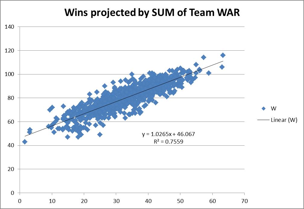
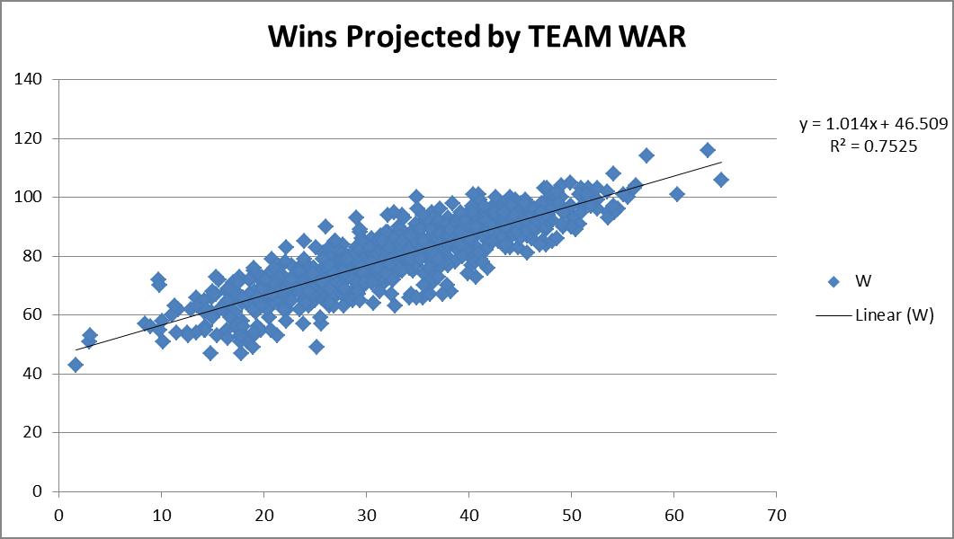
When I think of WAR, I tend to think of it truly in terms of wins.  So when I see that a player is rated an 8 WAR player, to me I’m literally thinking this guy will get my team approximately eight additional wins.  Otherwise we should really just rename this “best player metric.”  Not that anything is wrong with a best player metric, but let’s not try to “connect” it to wins, if it’s not really connecting to wins, right?  So I wanted to see how accurate this really is.  So I downloaded the team WAR data from FanGraphs from 1985 – 2013, both hitting and pitching. I summed up the hitting & pitching WAR and plotted them versus the teams’ wins that year, hoping for a strong correlation.

You can see from the chart above, a correlation of 0.7525 was recorded. Great! This also shows a replacement-level team is about a 46.5-win team.  Not unreasonable. Things make sense.
So then I figured, maybe we could try to do this same drill, but instead of using complete team calculations, what if we used individual position components?  Would that result in a more accurate result?  It’s possible, since the sum of a team’s individual player WAR values is not necessarily representative of the team WAR calculation alone.  So what would this look like?  So I went to FanGraphs again and downloaded the same dataset, except by position this time, instead of by team.  For example, I’ve linked the catcher data below.
I went through and built a comprehensive list, tagging each player’s position.  For pitchers the FanGraphs link was comprehensive, so I determined the RP and SP tag by assigning anybody who had >75% of their games also be games-started, as a SP, and all others as RPs.  In some cases players showed up in multiple categories (i.e. Mike Napoli was listed as a C and 1b in 2011).  In those events, I simply equally split their total seasonal WAR evenly across however many positions.  So if a 6 WAR player showed up as a C & 1b & DH in a single season, each position was credited with 2 WAR. This prevented double or triple-counting of players.  So how did this work out?
This actually projected slightly better. I do mean slightly — 0.7559 R2 versus the 0.7525 R2 when viewed as just team hitting and pitching.  It also predicted basically the same replacement-level team, a 46-win one.  So you could probably make the argument that it’s slightly more accurate to try to actually use the sum of the individual player WARs on the team instead of just a team calculation.  But it is so close it’s probably not worth the extra effort for most exercises.
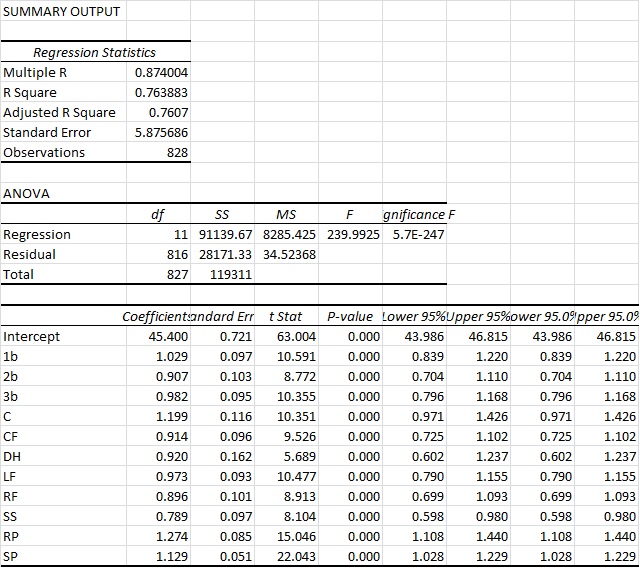
This then led me to think, why not try to tie wins in as a multi-variable regression using all the positions individually instead of just a linear one where we connect wins to some singular WAR total?
Since I already had the data i gave it a shot.
You can see here that we actually arrive at an R2 of a bit above 76%.  So this is ever so slightly more predictive again.  Again you also see that the intercept ends up very close to other methods, at 45.4 Wins for a replacement-level team.  But bottom line, it’s basically as accurate as the other approaches.  However, what I do find interesting in this approach is that it actually appears to value RP highest and the SS position the lowest.  And those values are substantial. Very substantial.
You could probably make the argument then that shortstops are being overvalued by the present system. This could possibly mean the defensive position adjustment value for SS defense is too high.  Reasons aside, this seems like a very legit finding, as the “WAR” metric appears to overstate SS value by 26.7% (1/0.789).  So for example, a typical FanGraphs contract analysis approach can use a standard $/WAR value for projections into the future. Yet from this perspective, spending that $/WAR on a SS will have you significantly overweighting the benefit you’ll get from that SS.  To a lesser extent that would also apply to 2b, CF and RFs.
Conversely, RP, SP and catcher figures are actually quite undervalued.  This would certainly lend some credence to the approaches of “smaller” and “rebuilding” teams to date (think Royals and Astros, even last year’s Yankees) who have focused, among other things, on RP groups.
Based on this data, it would seem that focusing on pitching, specifically RP, and getting an excellent catcher, would be the best ways to focus on turning around a team.  At least in the context of a singular $/WAR metric.
While this wasn’t what I went into this analysis looking for, it was a fairly surprising result. Yet one that seems to be in line with the approach many teams are currently taking.
NOTE: I do understand this could be refined even further to re-weight the players WAR values exactly correctly based upon their actual number of games at each position instead of the approach I took which was just to equally distribute those values.  Given the size of that specific sample and what type of change we’d be talking about, I would find it unlikely that would move the needle substantially here though. But I think it’s an interesting finding.

On the Use of Aging Curves for Fantasy Baseball

A question that tends to pop up around this time of year: “When does fantasy baseball season start?” Of course, we all know that fantasy-baseball season never ends, especially for those of us in keeper and dynasty leagues. To wit, Brad Johnson’s “Keeper Questions” thread posted just the other day is now sitting at 350 comments and growing. As we all collectively count the days ‘til spring training and opening day, one of the most oft-discussed and most subjectively-answered topics is “Who do I keep?” Fantasy baseball players intuitively understand the idea of aging, at least qualitatively. Older players are less valuable, given that their performance is more likely to decrease due to both injury and ineffectiveness. But how much is age worth, really?

Read the rest of this entry »


The Risk and Reward of Attempting to Pick Runners Off

Recently, Dave Cameron examined a planned back-pick by Russell Martin and the Blue Jays in Game 1 of the ALDS.  The play didn’t have a chance to happen because Delino DeShields put a 2-1 change up in play.  Not just in play, but on the ground to directly where the second baseman Ryan Goins would have been had he not been breaking for second in anticipation of the pick.  Dave wrote a great article that covered the play in depth, so feel free to go read it here.  In this article, I analyze the strategy of calling for a set pickoff attempt. What I found not only vindicates Martin and the Jays, but also questions one of my longest-held beliefs about pickoffs.

My strategy for evaluating the set pickoff was to calculate the break-even point (BEP) for a pickoff attempt using Run Expectancy (RE), similar to previous analyses on bunting and stealing. To calculate the BEP for a given pickoff attempt, I calculated the RE benefit (to the defense) of an out and the weighted RE cost of a safe call or an error.  This sounds simple enough, but calculating the RE after an error involved some guesswork.

Although errors can result in multiple outcomes, I chose to pick one outcome for each base to simplify the analysis. Thus, I assumed 2 bases for all runners on an errant throw to first, 1 base for all runners on an error to second, and, after much thought, 2 bases for runners on second and 1 base for runners on the corners on an error to third. If you have data that can replace these assumptions, please let me know.  Otherwise, be cognizant of my assumptions when you attempt to make use of the findings.  For example, if there is a slow runner on second, the BEP for a pickoff attempt to a corner will be overly conservative (inflated).  Additionally, I didn’t differentiate between pickoff attempts from the pitcher and the catcher.  The pitcher has a shorter, unobstructed throw, and favorable balk rules when picking to second or third, but still has to deal with the risk of a balk, especially to first, along with the added difficulty of throwing off the mound.  Finally, while calling for a back-pick from the catcher can put a defender out of position, I chose to ignore this factor because a) I assume it is rare for a hitter to find the vacated hole, and b) the defense can choose to avoid contact.

In order to weight the cost of a failed pickoff attempt appropriately, I had to estimate what the error rate would be on attempts.  While we do have data on pitcher error rates on pickoff attempts (around 0.95%), the data are only from throws to first.  Set pickoff plays are more challenging for the defense, so the error rate should be higher than on typical attempts to first.  My solution, in lieu of empirical data from actual set pickoff attempts, was to estimate catchers’ throwing error rates from the 2015 season.  I chose this strategy for two reasons: First, catchers are one of the primary players who can attempt a set pickoff, so it made sense to sample from their performance.  And second, catchers accumulate a large portion of their assists under similar conditions to the pickoff attempt (for example, in 2015 nearly 40% of all catcher assists came from caught stealing).  Thus, I expected catcher throwing error rates to approximate the error rates we would observe on set pickoff plays.

While not a perfect method, I estimated catcher throwing error rate as Throwing Errors / Assists + Throwing Errors + Stolen Bases.  The mean throwing error rate in a sample of catchers (n = 38) who played at least 500 innings in 2015 was 3.6%.  Do you accept that set pickoff plays will result in 3.8 times more errors than typical pickoff throws to first? If not, adjust your own estimates accordingly.

Using the estimated throwing error rate for catchers, the formula for estimating the BEP on a set pickoff attempt is RE cost / (RE cost – RE benefit). In this equation, RE benefit = RE after a pickoff – RE before a pickoff; RE cost = RE before a failed attempt – RE with a failed attempt, and RE with a failed attempt = (RE of a safe call *.964) + (RE of an error *.036).  Using the RE tables found here, I generated Table 1 below.


Runners Outs First Second Third
1 _ _ 0 3.51%
1 3.32%
2 3.24%
1 2 _ 0 3.32% 2.18%
1 4.21% 1.93%
2 9.17% 2.33%
1 _ 3 0 2.37% 0.74%
1 3.47% 1.92%
2 6.72% 5.99%
_ 2 3 0 1.70% 1.41%
1 1.93% 1.73%
2 5.06% 5.06%
1 2 3 0 10.21% 1.97% 1.64%
1 4.85% 2.78% 2.48%
2 7.58% 3.92% 3.92%
_ 2 _ 0 1.54%
1 1.43%
2 1.26%
_ _ 3 0 0.11%
1 1.74%
2 5.61%

Table 1.  Success rate required to attempt a pick at each base.

Table 1 presents the BEP for the defense of (successful pickoffs / attempts) X 100.  In other words, Table 1 provides the minimum expectation of success required for the defense to attempt a set pickoff and it be a break-even strategy. Unfortunately, it is difficult to guess how successful set pickoff attempts typically are.  In Dan Malkiel’s study of pickoffs to first, he found that righties and lefties were successful about 2% and 4% of the time, respectively.  However, Malkiel’s study sampled situations with base-stealers on first, so the stolen-base rate was between 17% and 21%.  It’s impossible to know what percentage of successful pickoffs occurred when the runner intended to steal, but it’s safe to say 2% and 4% success rates are a little high if the runner on first isn’t planning on going. Set pickoffs usually work differently than throws to first, since neither the pickoff nor the steal are always expected. Therefore, the data on picks to first can only serve as a point of reference, helping to calibrate expectations rather than serving as predictions themselves.

One way to assess if teams are over- or under-utilizing set pickoffs is to compare their pickoff to error ratios with the BEPs for that metric. Unfortunately, I could only find data for one special case of the set pickoff: a catcher back-pick to first.  In the Malkiel study, successful back-picks were 96% of back-picks plus errors.  If we assume an error puts the runner on third, the BEP for pickoffs/pickoffs + errors is 50%, suggesting that catchers have room to get much more aggressive in attempting to pick runners off first.  Without more data, it’s difficult to comment further on current MLB behaviour regarding set pickoff plays. Nevertheless, the estimates in Table 1 provide interesting insights into the risks and rewards of pickoff plays. Below, I list six lessons that can be gleaned from Table 1.  At least two of these lessons fly directly in the face of my own long-held beliefs, and maybe yours too!

Lesson 1

If, at any time, the defense notices that it has better than a 15% chance of picking off a runner, they should attempt the pickoff.

Lesson 2

Pickoff attempts require greater confidence with two outs, with three exceptions.  Often, the required success rate is over 5%, requiring a fairly egregious mistake by the runner to warrant a throw. The exceptions to this rule are with a runner on first, a runner on second, or a pick to second with runners on first and second.

Lesson 3

A runner on second with no runner ahead of him should probably be targeted frequently.  The BEPs are consistently low for attempting the pickoff to second, while the runner is motivated to be aggressive by the chance to score a run or steal third. Even failed attempts have the favorable by-product of keeping the runner close, a factor not considered in Table 1.

Lesson 4

Throwing behind the runner on first with runners on first and second or the bases loaded is dangerous.  This doesn’t mean it’s a bad play if the runner on first opens the door, but the defense should be really confident to make the throw.

Now for the lessons that go against everything I thought I knew…

Lesson 5

Pitchers should throw over to third with runners on 1st and 3rd in a steal situation.  Ever since the MLB outlawed the fake-to-third move, pitchers haven’t been allowed to bluff the throw in hopes of catching the runner breaking from first.  Based on Table 1, it seems strange that pitchers ever faked the throw to begin with.  With no one out, the defense would only need to pick the runner off third 8 times per 1000 attempts, or nail the runner stealing second 3 times per 100 attempts, or a combination of the two to break even.  Additionally, if the runner on first breaks for second it’s an easier throw from third than from first, which was often the result with the fake-to-third move.  While many old-school baseball people will object to throwing over to third, the common refrain “he’s not going anywhere!” doesn’t necessarily apply to the 1st and 3rd steal situation.  The runner could be trying to get closer to home so he can steal on the catcher’s throw to second, making it the perfect time to throw over.  Although the third baseman’s positioning will sometimes make a true pickoff attempt at third difficult, the rules do not require the pitcher to throw directly to third.  Thus, teams can make legitimate efforts to get the runner on third when the situation allows it, while other times making throws away from the base solely to catch the runner on first breaking for second.

Lesson 6

The situation that requires the lowest probability of success to attempt a pickoff is when there is a runner on third with no one out.  The defence needs to nab merely 2 runners out of every 1000 attempts to break even. And get this, the BEP on pickoff attempts to third with 0 out is lower than the BEP for typical throws to first, even with the much lower error rate on throws to first (0.95%), and even after adjusting the assumed cost of an error to one base.  Holding probability of success constant, the pickoff attempt to get a runner on third with 0 out is the least risky pickoff attempt possible. The LEAST risky.

Of course, a runner who is on third with no one out should be taking no chances.  But that doesn’t mean a pickoff will never work…


How Game Theory Is Applied to Pitch Optimization

The timeless struggle between pitcher and batter is one of dominance — who holds it and how. Both players use a repertoire of techniques to adapt to each other’s strategies in order to gain advantage, thereby winning the at-bat and, ultimately, the game.

These strategies can rely on everything from experience to data. In fact, baseball players rely heavily on data analytics in order to tell them how they’re swinging their bats, how well they’ll do in college, how they’ll perform at Wrigley versus Miller.

Big data has been used in baseball for decades — as early as the 60s. Bill James, however, was the first prominent sabermetrician, writing about the field in his Bill James Baseball Abstracts during the 80s. Sabermetrics are used to measure in-game performance and are often used by teams to prospect players.

Baseball fans familiar with sabermetrics, the A’s, and Brad Pitt have likely seen Moneyball, the Hollywood adaptation of Michael Lewis’ book. The book told the story of As manager Billy Beane’s use of sabermetrics to amass a winning team.

Sabermetrics is one way baseball teams use big data to leverage game theory in baseball — on a team-wide scale. However, by leveraging their data through the concepts of game theory on a smaller scale, baseball teams can help their men on mound out-duel those at the plate.

Game theory studies strategic decision making, not just in sports or games, but in any situation in which a decision must be made against another decision maker. In other words, it is the study of conflict.

Game theory uses mathematical models to analyze decisions. Most sports are zero-sum games, in which the decisions of one player (or team) will have a direct effect on the opposing player (or team). This creates an equilibrium which is known as the Nash equilibrium, named for the mathematician John Forbes Nash. What this means is that if a team scores a run, it is usually at the expense of the opposing team — likely based on an error by a fielder or a hit off a pitcher.

In the case of pitching, game theory — especially the use of the Nash equilibrium — can be used to predict pitch optimization for strategic purposes. Neil Paine of FiveThirtyEight advocates using big data and sabermetrics to analyze each pitch in a hurler’s armory, then cultivating the pitcher’s equilibrium — the perfect blend of pitches that will result in the highest number of strikeouts, etc.

Paine has gone so far as to create his own formula, the Nash Score, to predict which pitcher should throw which pitches in order to outwit batters.

In perfect game theory, the Nash equilibrium states that each game player uses a mix of strategies that is so effective, neither has incentive to change strategies. For pitchers, Paine’s Nash Score uses their data to find the optimal combination of pitches to combat batters, including frequency.

Paine does point out that creating this kind of equilibrium in baseball can be detrimental to a pitcher. He is, after all, playing against another human being who is just as capable of using game theory to adapt strategies to upset the equilibrium.

If a pitcher’s fastball is his best, and his Nash Score shows that he should be using it more often, savvy hitters are going to notice. “ . . . In time, the fastball will lose its effectiveness if it’s not balanced against, say, a change-up — even if the fastball is a far better pitch on paper,” writes Paine.

In this case, a mixed strategy is the best — in game theory, mixed strategies are best used when a player intends to keep his opponent guessing. Though pitch optimization using Paine’s Nash Score could lead to efficiency, allowing pitchers to throw fewer pitches for more innings, it could also lead to batters adapting much quicker to patterns, thus negating all the work.


Where to Bat Your Best Hitter: A Computational Analysis (Part 1)

Prior to the August, 2015, non-waiver trade deadline, the Toronto Blue Jays sent their leadoff hitter Jose Reyes to the Colorado Rockies for Troy Tulowitzki, a classic middle-of-the-order bat. Everyone assumed from his career power numbers that Tulowitzki would slot in the heart of the Jays order, but with Josh Donaldson, Jose Bautista, and Edward Encarnacion already comfortably set at 2-4 (over 200 RBIs between them at the time) they instead used him in the vacated leadoff spot. The move seemed to work as Tulo went 3 for 5 in his first game, and the Jays proceeded to rattle off a tidy 11-0 streak with their new top-of-the-order guy.

Troy Tulowitzki
Shortstop B/T: R/R
.297 / .370 / .510
29 HR 100 RBI 8 SB
TT José Reyes
Shortstop B/T: B/R
.290 / .339 / .432
12 HR 65 RBI 50 SB
JR

One doesn’t mess with success, but everyone knows Tulowitzki is not an ideal leadoff hitter, never having batted there before in his 10-year MLB career, and with all of 3 stolen bases in the last 3 seasons. His above-average pop suggests a traditional run-producing spot: 29 HR and 100 RBI career numbers over an averaged 162-game season (Baseball-Reference.com), but with the Jays on a 22-5 tear, Tulo, touch wood, wasn’t moving anywhere.

A leadoff hitter naturally gets more at bats per season, one reason Jays manager John Gibbons gave for putting Tulowitzki at the top of the order, given his career .297 BA and .370 OBP. But tradition and common sense dictate that top RBI men are more valuable with men on base, impossible for a leadoff man in the first inning, and presumably sub-optimal afterwards. As Tulowitzki’s new teammate 3B Josh Donaldson noted in the midst of an August run that saw the Jays go from 6 back of the Yankees to 1 1/2 up in the AL East, “I feel like every time I’m coming up I have someone in scoring position or someone on base.” Exactly.

Fine-tuning a lineup is an argument for the ages, but can we determine where a power hitter should bat, where his numbers best fit 1 to 9? Should high-average batters hit before the sluggers, or should we just bat 1-9 in order of descending batting average (or OBP)? Can we calculate how to arrange a team’s lineup to maximize the optimum theoretical run production?

Enter Monte Carlo simulations, used to model the motion of nuclei in a DNA sequence, temperatures in a climate-change projection, even determine the best shape and size of a potato chip. In Do The Math!, Monte Carlo simulations were used to calculate where a Monopoly player will most likely land (Jail and Community Chest, followed by the three orange properties: St James, Tennessee, and New York), and whether to hit or stick in Black Jack against any dealer’s up card.

In some cases, algebraic probabilities are difficult (using Markov chains, a continuously iterative system with a finite countable sample space), whereas brute force computation does the trick over a large number of trials. If a picture is worth a thousand words, a simulation is worth a thousand pictures.

BOO V1 (Batting Order Optimization Version 1) is a Monte Carlo program written in Matlab that randomly selects a hit/out event over a 9-inning, 27-out game, averaged over a large number of games, e.g., 1 million. It uses a flat lineup where all hitters have a .333 OBP (roughly the Jays average), but doesn’t include errors, hit batsmen, sacrifices, double plays, stolen bases, etc., or opposing pitchers’ numbers. (In Part II, I will include the hitting stats of a real lineup: 1B, 2B, 3B, HR, BB, K, GO/AO.)

The mathematical guts are fairly simple, essentially a random number generator and some modulo math (think of leap-frogging 3 or more chairs at a time in a circle of 9), and elegantly captures some interesting trends, in particular, the distribution of end-game batters 1-9 and thus the most likely batter to end a game. From such a simulation, we can calculate where best to slot a team’s best hitter to maximize his chances of coming to the plate with the game on the line, another stated reason for putting Tulo in the Blue Jays number 1 spot.

Figure 1a shows the distribution of batters faced (BF) over 1,000,000 simulated BOO games, where the most likely end was 40 batters faced followed by 39 and 41 (the 3-5 hitters), as might be expected with a hard-wired OBP = .333 (binomial p = .33). It seems the custom of having your clutch hitters in the 3-5 slots matches the computational results.
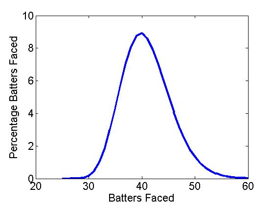
BOOFigure1a BOOFigure1b

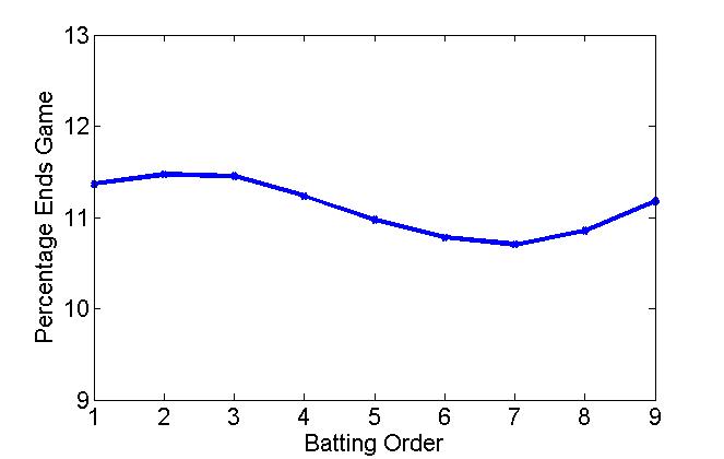
Figure 1a: Distribution of # of batters faced   Figure 1b: Distribution of end-game batters

Interestingly, however, the leadoff hitter doesn’t end a game more often than a middle-order batter. Figure 1b shows the distribution of end-game batters (EGB) for a 1-9 lineup, and is perhaps counter-intuitive. In fact, the number 2 and 3 hitters are more likely to end a game than the leadoff hitter, while there is an obvious dip 3-7. Table 1 shows the frequency of end-game batters 1-9 (number and percentage).

1 2 3 4 5 6 7 8 9
# of games ended 18.4 18.6 18.6 18.2 17.8 17.5 17.3 17.6 18.1
% games ended 11.4 11.5 11.5 11.2 11.0 10.8 10.7 10.9 11.2

Table 1: Number of games ended and percentage versus lineup position (OBP = .333)

Initially, I expected a constant drop-off from 1 to 9, or perhaps following some form of a Benford’s Law distribution, for example, in the wear pattern on a ATM pad or the leading digit in a collection of financial data (1 appears about 30%, 2 about 18%, 3 about 12%, 4 about 10%, . . . , and 9 about 5%). Note, if the data were randomly distributed, each number would appear 11.1% or 1/9. But the modulo aspect of a repeated baseball lineup creates another distribution, one that has a clear maximum after the leadoff spot and a mid-lineup dip at batter number 7.

Of course, the leadoff hitter will always have more plate appearances over an entire season, but somewhat surprisingly does not end a game more often. Table 2 shows the number of at bats 1-9 averaged over a 162-game season (I have assumed 8.5% of plate appearances are walks). As can be seen, the leadoff hitter gets about 130 more ABs than the number 9 hitter, or 21% more per season, reason enough to put your best hitter at the top of the order. From one batter to the next, however, the difference is only about 17 ABs (monotonically decreasing), about an extra AB every 10 games. Not that much difference one spot to the next.

1 2 3 4 5 6 7 8 9
# of ABs 757 740 723 706 689 673 657 641 625
% ABs 12.2 11.9 11.6 11.4 11.1 10.8 10.6 10.3 10.1

Table 2: Number of ABs and percentage ABs over 162 games (OBP = .333)

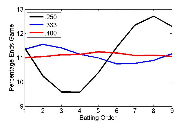
Using BOO, we can also analyse how the EGB distribution changes for a good and a bad team, modelled using an OBP of .250 and .400. The results are shown in Figure 2 including our .333 OBP team. Here, it seems that the lineup order matters more on a bad team than a good team (a practically flat EGB). Indeed, it is often said that you can run any lineup out with a good team. Conversely, losing teams are always juggling their lineups to find the right mix.
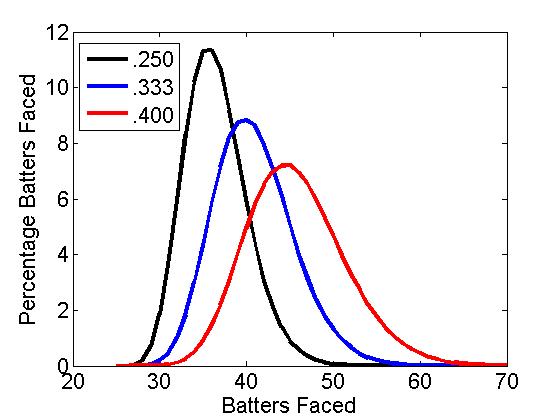
BOOFigure2a BOOFigure2b

Figure 2a: Distribution of # of batters faced   Figure 2b: Distribution of end-game batters (OBP = .250, .333. .400)

Of course, baseball is not just statistics over a large number of sample-sizes (or simulations). Baseball is played in bunches and hunches. It would take a little over 400 years to play 1,000,000 games in a 30-team, 162-game schedule. Matchups, streaks, situational hitting, and team chemistry may be more important than any theoretical trends. And, of course, a real, non-flat, batting lineup (which I’ll look at in Part II).

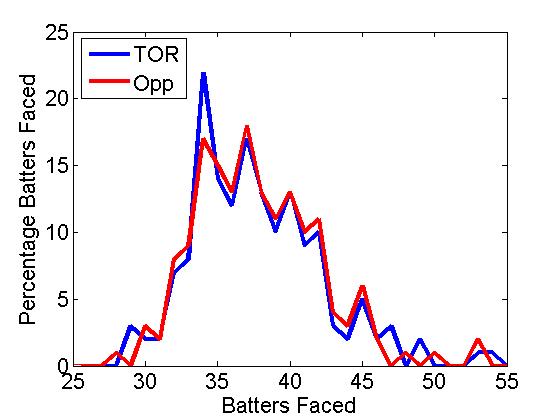
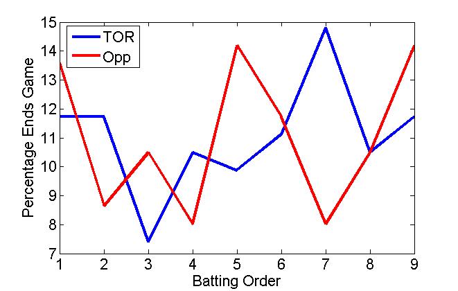
In an actual BF and EGB distribution for the 2014 Toronto Blue Jays and their opponents over a 162-game season, we see the small-sample versions of our super-sized theoretical distributions (Figure 3). The actual BF distribution is comparable to the theoretical binomial/Gaussian BF, though positively skewed, showing the effect of blowouts, not adequately covered in the hit/out simulation. The EGB distribution seems quite random, but late peaks may indicate the use of pinch hitters in the closing parts of a game. It is also interesting to note that BOO “throws” a perfect game about once every 10 seasons, a bit less than the official 23 over the last 135 years.
BOOFigure3a BOOFigure3b

Figure 3a: Distribution of # of batters faced   Figure 3b: Distribution of end-game batters (2014 Toronto Blue Jays and opposition)

So do the calculations mean anything? According to the numbers, your best hitter should bat 2 or 3, that is, if you want him coming up more often with the game on the line. In “The Batting Order Evolution,” Sam Miller noted that “the anecdotal evidence is strong” to put your best hitter in the number 2 spot. The worst spot for heroics is number 7.

Furthermore, a classic run producer such as Troy Tulowitzki shouldn’t bat leadoff, something the Jays found out after he struck out 4 times, almost a month to the day after acquiring him. Dropping him to the number 5 spot, the manager John Gibbons stated, “Maybe this’ll jump-start him a little bit.” Or maybe, he saw the wisdom of inserting the 2014 NL hit leader and speedster Ben Revere in the leadoff spot and using Tulowitzki’s power in a proven RBI position.

Mind you, with a scorching hot lineup that has scored 100 more runs than the next-best hitting team, it may not matter who bats where. That is, if the game is on the line.

Do The Math! is available in paperback and Kindle versions from the publisher Sage Publications, on-line at Amazon.com, and on order at local book stores. Do The Math! (in 100 seconds) videos are on You Tube.


Searching for Dexter Fowler(s): Finding Value in Fantasy Baseball

If Dexter Fowler or any of the other Dexter Fowler-type players mentioned below are sitting on your fantasy baseball waiver wire, then stop what you’re doing right now and snag them. What follows mainly applies to deeper mixed-leagues, but frankly, I’m a little tired of reading the musings of “experts” on how this or that guy is “viable only in NL-only” or “shallow-mixed” leagues. That’s all well and good, but let’s cut the crap: we want guys who produce counting stats, and Dexter Fowler and those like him do precisely that for leagues big and small. They score runs, steal bases, hit home runs, get on base, and more, but for some reason, people don’t give them the credit they deserve. For instance, Fowler, with his 10 HR, 66 R, and 16 SB, just finally cracked the ESPN Top-250 list this past week; but he’s still ranked behind the likes of Logan Morrison. See what I mean? But I digress.

Here’s my point: If you’re like me — and you probably are, to the extent that you love playing Rotisserie/fantasy baseball — then you’re looking to find value on the waiver wire or via trade; you’re looking for undervalued players who produce counting stats. Sounds easy enough, and if you look at the ownership rates of a few guys I’m particularly keen on, then it really is easy to find these guys free of charge; guys like Dexter Fowler (owned in 57% of ESPN leagues), David Peralta (27%), Preston Tucker (27%), or Marlon Byrd (34%). Are these names flashy? No, not really, but who cares; they produce.

There are plenty of other, similar players who all have a few things in common relevant to us baseball-minded folk: they produce in at least three categories and are probably on your waiver wire or sitting on someone’s bench ripe for a trade offer from you. Why these players — and those like them — are so under-owned is, in many cases, the result of playing time (i.e., platoons), but I also suspect the ownership percentages are skewed by 8-team leagues . In deeper leagues, however, like those I care about, Dexter Fowlers are must-haves.

Here’s at look at how the Dexter Fowlers I’ve identified (and there are many more) can help you. I’ve also provided some stats and thoughts on why so few people have grabbed these particular guys. In any case, these are guys you’ll want down the stretch.

Dexter Fowler: How many guys have double-digit home runs and stolen bases in MLB this year? Eighteen. 18! Fowler, recall, was once a highly touted prospect in the Rockies organization, and while he never quite turned into the superstar many had projected, he has had a fine career, and hitting in front of Kris Bryant and Anthony Rizzo (and lately, ahem, Chris Coghlan) is helping Fowler have one of his finest seasons to date. Currently on pace to destroy his single-season career high homer total of 13 set in 2012, Fowler is also on pace for his first 20 SB season since his rookie year, while remaining among the league leaders in runs scored (currently 4th in the NL at 66).

Let’s take a step back for a second: Fowler has 10 HR and 16 SB. That’s fantastic in its own right, but he gets zero love (or 57% love, as it were). The knock on Dexter, of course, is his low batting average. However, that argument is starting to fall apart, as the average is on the rise and it’s been dragged down by a career-low .297 BABIP (career BABIP of .342). Not to mention Fowler takes a ton of walks, thus helping buoy his run and stolen base totals in the absence of hits. And on top of the great counting stats and rising average, Fowler is a switch hitter, leaving him immune to benching in the face of tough lefty/righty matchups.

For perspective, consider this: Christian Yelich is ranked ESPN’s number 35 outfielder for Roto 5×5 leagues (117 player overall); Fowler is ranked OF #59 (230 overall). Here are their stats; I have no idea what drugs ESPN is taking, but I want some.

Yelich (owed in 67%): .263; 35 R; 6 HR; 25 RBI; 10 SB (note: he did spend roughly three weeks on the DL and is without the benefit of Stanton)

Fowler: .243; 66 R; 10 HR; 27 RBI; 16 SB.

Here’s more perspective: According to ZiPS projections, Yelich is on pace to finish the season with stats in all categories almost identical to what Fowler has achieved by July.

Why the disparity in rankings? You tell me — potential, I suspect, but you don’t need a PhD in statistics to tell you that Fowler is vastly outperforming Yelich this year, and we are well beyond the days where the small-sample size caveat holds water. Yelich, to his credit, is a fantastic hitter and has a bright career ahead of him, but he’s got nothing on Dexter Fowler in 2015.

Here are a few other Fowler-types to keep in mind:

David Peralta: The dude crushes right-handed pitching. Peralta, a converted pitcher, has an average batted-ball velocity of approximately 95 MPH according to baseballsavant.com (that’s really, really good). He currently owns a .281/.351/.493 triple slash with 9 HR and 48 RBI, though he rarely plays against lefties (which is perhaps stupid, but a topic for another time) despite a recent vote of confidence by Chip Hale for his improved ability to mash lefties as well.

Bottom line: Peralta flat-out hits. He’s been on a roll since Inciarte went on the DL, and thanks to the maddening way in which Hale manages his lineup, Peralta is not an everyday starter — but against righties, which make up the majority of National League pitching (by far), Peralta holds prime real estate in Arizona’s lineup and should be in your lineup as well, and ahead of guys like, for instance, Christian Yelich. And maybe even Dexter Fowler, depending on your particular needs. In addition to Peralta’s 9 HRs in 288 ABs, he’s also stolen five bases and regularly slots in the 2-hole when he’s not batting cleanup.

In a stacked Arizona lineup, opportunities to score and drive in runs are plentiful — as he’s shown over the past two months. If nothing else, just bench him against lefties and start him against righties, whom he absolutely destroys, which reminds me of Preston Tucker.

Preston Tucker: A highly regarded prospect in the Astros organization, Tucker was called up from Fresno in May. He got off to a hot start, cooled in June, but here in July/August, Tucker is again raking. Known as “Bam Bam” for his likeness to Fred Flintstone’s pal (or grandfather?), Tucker is 25 and has crushed 77 homers (minors & majors) since 2012, after being a 7th round pick in 2012. His platoon splits aren’t pretty; you won’t want to start him against the few lefties he’s allowed to face, but what he does to righties almost makes me feel bad for the pitchers: He’s slashing .296/.356/.568 against righties (OPS of .924 if you don’t like math), with 5 HR in 46 AB’s since the All-Star break.

Start Tucker with confidence; he bats second or cleanup against righties, and with Gomez in town, Jake Marisnick (a righty) is the odd man out more often than not — Tucker and his .924 OPS do too much damage to bench against RHP. Also note that Tucker gets more starts than does Colby Rasmus (until the return of Springer, when they both likely sit) another guy I like, incidentally, for his power vs. righties. Tucker’s power is real; his ISO is a lovely .204 and his .265 batting average aligns well with his minor league numbers, and his BABIP is a sustainable .299 given his hard-contact rate and minor league numbers.

Marlon Byrd: He’s hit 18 home runs and, in his last 60 games (roughly), is hitting over .290 with 15 home runs. He’s owned in 34% of ESPN leagues. Byrd has hit 25 and 24 homers the past two years, respectively. Enough said.

As I mentioned, there are plenty of other Fowlers out there, and I will cover those in my next post. Hint: Gerardo Parra (72%!); Colby Rasmus (5%); Jarrod Dyson (7%).


A Discrete Pitchers Study – Out & Base Runner Situations

(This is Part 4 of a four-part series answering common questions regarding starting pitchers by use of discrete probability models. In Part 1 we explored perfect game and no-hitter probabilities, in Part 2 we further investigated other hit probabilities in a complete game, and in Part 3 we predicted the winner of pitchers’ duels. Here we project the probability of scoring at least one run in various base runner and out scenarios.)

V.  I Don’t Know’s on Third!

Still far from a distant memory, the final out of the 2014 World Series was preceded by an unexpected single and a nerve-racking error that brought Alex Gordon to 3rd base with two outs. Closer Madison Bumgarner, who was on fire throughout the playoffs as a starter, allowed the hit but would be left in the game to finish the job. There is some debate as to whether Gordon should have been sent home rather than stopped at 3rd base , but it would have taken another error overshadowing Bill Buckner’s to get him home; also, next up to bat was Salvador Perez, the only player to ever ding a run off Bumgarner in three World Series. So even though the Royals’ 3rd Base Coach Mike Jirschele had to make a spur of the moment critical decision to stop Gordon as he approached 3rd base, it was a decision validated by both statistics and common sense. We will show our own evidence, by use of negative multinomial probabilities, of how unlikely the Royals would have scored the tying run off of Bumgarner with a runner on 3rd with two outs and we will also consider other potential game-tying or winning situations.

Runs are generally strung together from sequences of hits, walks, and outs; in the situations we will consider, we will only focus on those sequences that lead to at least one run scoring and those that do not. Events not controlled by the batter in the box, such as steals and errors, could also potentially reshape the situation and lead to runs, but we’ll take a very conservative approach and assume a cautious situation where steals are discouraged and errors are extremely unlikely.

Let A and B be random variables for hits and walks and let P(H) and P(BB) be their respective probabilities for a specific pitcher, such that OBP = P(H) + P(BB) + P(HBP) and (1-OBP) is the probability of an out; we combine the hit-by-pitch probability into the walk probability, such that P(BB) is really P(BB) + P(HBP) because we excluded hit-by-pitches from our models, P(HBP) > 0 against Bumgarner in the 2014 World Series, and the result on the base paths is the same as a walk. The first negative multinomial probability formula we’ll introduce considers the sequences of hits, walks, and an out that can occur after two outs have been accumulated, setting the hypothetical stage for the last play in Game 7 of the 2014 World Series.

Formula 5.1

In the 2014 World Series, Bumgarner’s dominantly low P(H) and P(BB) were respectively 0.123 and 0.027 and his (1-OBP) was 0.849; by applying these values to the formula above we can generate the probabilities of various hit and walk combinations shown in Table 5.1. The yellow highlighted cells in the table represent the combination of hits and walks that would let Bumgarner escape the inning without allowing the tying run (given a runner on 3rd with two outs and a one run lead). By combining these yellow cells, we see that the odds were overwhelmingly in in Bumgarner’s favor (0.873); all he had to do was get Perez out, walk Perez and get the next batter out, or walk two batters and get the third out.

Table 5.1: Probability of Hit and Walk Combinations after 2 Outs

0 Hits 1 Hit 2 Hits 3 Hits 4 Hits
0 Walks 0.849 0.105 0.013 0.002 0.000
1 Walk 0.023 0.006 0.001 0.000 0.000
2 Walks 0.001 0.000 0.000 0.000 0.000
3 Walks 0.000 0.000 0.000 0.000 0.000
4 Walks 0.000 0.000 0.000 0.000 0.000

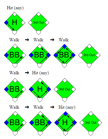
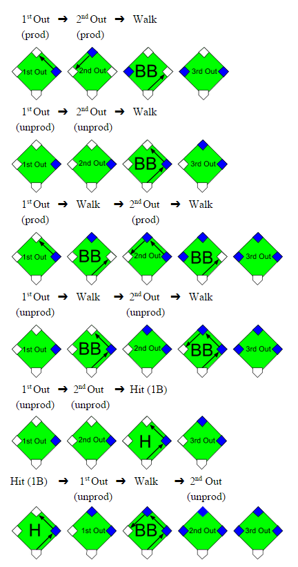
The Royals could have contrarily tied the game with a simple hit from Perez given the runner on 3rd and two outs, yet this wasn’t the only sequence that would have kept the Royals hopes alive. Three consecutive walks, one walk and one hit, or any combination of walks and one hit could have also done the job; examples of these sequences are shown in the graphics below:

Graphic 5.1

Generally, any combination of walks and hits not highlighted yellow in Table 5.1 would have tied or won the World Series for the Royals. This glimmer of hope was a quantifiable 0.127 probability for Kansas City, so it was justified that Gordon was kept at 3rd rather than sent home after shortstop Brandon Crawford just received the ball. It would have taken an error from Crawford or Buster Posey, with respective 0.033 and 0.006 2014 error rates, to get Gordon home safely. The probability 0.127 of winning the game from the batter’s box is noticeably three times greater than the probability of winning it from the base paths (where Crawford and Posey’s joint error probability was 0.039).

We should note that the layout in Table 5.1 is a simplification of what could occur with a runner on 3rd, two outs, and a one run lead, because it only applies to innings where a walk off is not possible. In innings where a walkoff can occur, such as the bottom of the 9th, the combinations of walks and hits captured in the red highlighted cells are not possible because they would occur after the winning run has scored and the game has ended. However, Bumgarner was so dominant in the World Series that these probabilities are almost non-existent, thereby making our model is still applicable; we would otherwise exclude these red-celled probabilities for less successful pitchers.

The next probability formula considers the sequences of walks, hits, and outs that can occur after one out has been accumulated, which is situation definitely worth examining if there is a lone runner on 2nd base.

Formula 5.2

Once again we’ll use Bumgarner’s 2014 World Series statistics to evaluate this formula and insert the probabilities into Table 5.2. According to the sum of the yellow cells, Bumgarner would be able to prevent the tying run from scoring (from 2nd base with one out) with a probability of 0.762 and would otherwise allow the tying run with a probability of 0.238.

Table 5.2: Probability of Hit and Walk Combinations after 1 Out

0 Hits 1 Hit 2 Hits 3 Hits 4 Hits
0 Walks 0.721 0.178 0.033 0.005 0.001
1 Walk 0.040 0.015 0.004 0.001 0.000
2 Walks 0.002 0.001 0.000 0.000 0.000
3 Walks 0.000 0.000 0.000 0.000 0.000
4 Walks 0.000 0.000 0.000 0.000 0.000

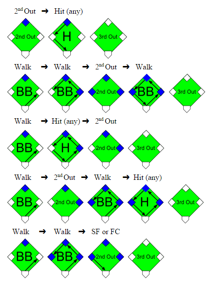
To get out of the inning unscathed, Bumgarner would need to prevent any further hits or allow fewer than 3 walks given a runner on 2nd with 1 out; it would be possible to advance the runner to on 3rd with 2 walks and then sacrifice him home in this situation (with no hits), but this probability is insignificantly tiny especially for a dominant pitcher like Bumgarner. Once again we depict these sequences that could get the tying run home from 2nd with 1 out, with the second out inserted randomly.

Graphic 5.2

A runner on 2nd base with one out is a scenario commonly manufactured in an attempt to tie the game from a runner on 1st with no outs situation. The logic is that if the hitting team is down by one run and the first batter leads off the inning with a single or walk, the next batter can control getting him into scoring position and hope that either of the next two batters knocks the run in with a hit. However, this method of control, a bunt, sacrifices an out to move the runner from 1st to 2nd. The defense will usually allow the hitting team to move the runner into scoring position for an out, but the out wasn’t the only sacrifice made. The inning is truncated for the hitting team with one less batter and the potential to have more hitters bat and drive in runs is reduced. Indeed, against a pitcher like Bumgarner, the out is likely not worth the meager 0.238 probability of getting that runner home.  We’ll see in the next section what exactly gets sacrificed for this chance at tying the game.

We should note that in this “runner on 2nd with 1 out” model we added few more assumptions to those we made in the prior “runner on 3rd with 2 outs” model, neither of which should be farfetched. The first assumption is that with the game close and the manager intent on tying the game rather than piling on runs, he should have a runner on 2nd base fast enough to score on a single. Another assumption is that the base runners will be precautious enough not to cause an out on the base paths, yet aggressive enough not to get doubled up or have the lead runner sacrificed in a fielder’s choice play. Lastly, we assume that the combinations of hits, walks, and outs are random, even though we know the current state of base runners and outs can have a predictive effect on the next outcome and the defensive strategy used. By using these assumptions we simplify the factors and outcomes accounted for in these models and reduce the variability between each model.

The final probability formula considers the sequences of walks, hits, and outs that can occur when we start with no outs accumulated; this allows to forge situation will allow us to forge the outcomes from a runner on 1st with no outs scenario and compare them to a runner on 2nd with 1 out scenario.

Formula 5.3

Table 5.3 below uses Bumgarner’s 2014 World Series statistics, the same as before, although in this model we deal with more uncertainty because the sequences captured in each box are not as clear cut between run scoring or not given a runner on 1st with no outs. The yellow and non-highlighted cells are still the respective probabilities of not allowing and allowing the tying run to score, however, we now introduce the green probabilities to represent the hit and walk combinations that could potentially score a run but are dependent on the hit types, sequences of events, and the use of productive outs. These factors were unnecessary in the prior two models because in those models any hit would have scored the run, the sequence of events was inconsequential, and the use of productive outs was unnecessary with the runner is already on 2nd or 3rd base (except when there is a runner on 3rd and a sacrifice fly or fielder’s choice could bring him home).

Table 5.3: Probability of Hit and Walk Combinations after 0 Outs

0 Hits 1 Hit 2 Hits 3 Hits 4 Hits
0 Walks 0.613 0.227 0.056 0.011 0.002
1 Walk 0.050 0.025 0.008 0.002 0.000
2 Walks 0.003 0.002 0.001 0.000 0.000
3 Walks 0.000 0.000 0.000 0.000 0.000
4 Walks 0.000 0.000 0.000 0.000 0.000

We must break down each green probability into subsets of yellow probabilities representing the specific sequences that would not score the tying run from 1st base with no outs; we depict these sequences below, but for simplicity, not all are depicted.

Graphic 5.3

Now that we know the conditions when a run would not score, we take the probabilities from the green cells in Table 5.3, narrow them down according to the proportion of sequences and the proportion of hit types that would not score the run, and separate them based on the usage of productive and unproductive outs; the results are displayed in Table 5.4. For example, there are 6 possible combinations for 1 hit, 1 walk, and 3 outs and 3 of these 6 combinations would not score the tying run on a single, where P(1B | H) = 0.755, with unproductive outs; yet, the run would score with productive outs, with unproductive outs on a double or better, or with unproductive outs and the other 3 combinations. When we finally sum these yellow cells, they tell us that an aggressive manager would score the tying run against Bumgarner with a 0.370 probability and Bumgarner would escape the inning with a 0.630 probability. Otherwise, a less aggressive manager would score the tying run with a mere 0.154 probability and Bumgarner would leave unscathed with a significant 0.846 probability.

Table 5.4: Probability of No Runs Scoring after 0 Outs

Productive Outs Unproductive Outs
0 Hits 1 Hit 0 Hits 1 Hit
0 Walks 0.613 x (1/1) 0.227 x (0/3) 0.613 x (1/1) 0.227 x (3/3) x 0.755
1 Walk 0.050 x (1/3) 0.025 x (0/6) 0.050 x (3/3) 0.025 x (3/6) x 0.755
2 Walks 0.003 x (2/6) N/A 0.003 x (6/6) N/A

We summarize the results from Tables 5.1-5.4 into Table 5.5 from the perspective of the hitting team.  We compare their chances of success not only against Madison Bumgarner from the 2014 World Series but also against Tim Lincecum, Matt Cain, and Jonathan Sanchez from the 2010 World Series.

Table 5.5: Probability of Allowing at least One Run to Score

2010 Tim Lincecum 2010 Matt Cain 2010 Jonathan Sanchez 2014 Madison Bumgarner
Runner on 1st & 0 Outs w/Unproductive Outs 0.305 0.224 0.531 0.154
Runner on 1st & 0 Outs w/Productive Outs 0.576 0.475 0.758 0.370
Runner on 2nd & 1 Out 0.382 0.288 0.543 0.238
Runner on 3rd & 2 Outs 0.212 0.154 0.318 0.127

Let’s return to the scenario that is the launching point for this study… The hitting team is down by one run and there is a runner on 1st base with no outs. If the game is in its early innings, where it is not mandatory that this runner at 1st gets home, the manager will likely decide against being aggressive and avoid sacrificing outs in order to increase his chances of extending the inning to score more runs; there are several studies supporting this logic. Yet, if the game is in the latter innings and base runners are hard to come by, the manager should lean towards utilizing productive outs and intentionally sacrifice the runner from 1st to 2nd base. His shortsighted goal should only be to tie the game.  By forcing productive outs rather than being conservative on the base paths, his chances of tying the game increase significantly (between 0.216 and 0.271) against our four pitchers given a runner on 1st and no outs scenario.

However, the if the manager does successfully orchestrate the runner from 1st to 2nd base with a productive out, he does still lose a little bit of probability of tying the game; between 0.132 and 0.215 of probability is lost against our pitchers. And if he decides to sacrifice the runner further from 2nd to 3rd base with another out, his team’s chances would decrease again by a comparable amount; this decision is ill-advised because a hit is likely going to be needed to tie the game and the hitting team would be sacrificing one of two guaranteed chances to hit in this situation. In general, the probability of scoring at least one run decreases as more outs are accumulated, regardless of the base runners advancing with each out. The manager could contrarily decide against sacrificing his batter if he has confidence that his batter can hit the pitcher or draw a walk, yet the imperative goal is still to tie the game. The odds of tying the game actually favor an aggressive hitting team that is able to get the runner to 2nd base with one out, by an improvement ranging from 0.012 to 0.084, over a less aggressive team with a runner at 1st with no outs. Thus, even though sacrificing the runner from 1st to 2nd base does decrease the chances of tying the game, it would be worse to approach the game lifelessly when the situation demands otherwise.


Replacing Replacement Value in Fantasy Auctions

With the baseball season rapidly approaching and recent posts by FanGraphs authors converting projected statistics into auction values, I thought I would share my approach towards valuation I have used in a long-standing A.L. league with 12 teams, 23 player rosters selected through auction (C, C, 1B, 3B, CI, 2B, SS, MI, 5 OF, 1 DH), a $260 budget, a 17-player reserve snake draft and the ability to keep up to 15 players from one year to the next, an attribute that inflates the value of the remaining pool and can further distort disparate talent across positions and categories.

We have traditionally used a 4×4 format, and while I have persuaded my co-owners to switch to a 5×5 for the coming year, what follows is my process for a 4×4 league.

There was a distant time when I was a whiz at math but my utter lack of a work ethic for advanced math collided with university-level calculus and I crumbled as surely as a weak-kneed lefty facing Randy Johnson. So my understanding of some key statistical processes is compromised. And by some I mean most.

But what I lack in math I hope I make up in approach:

(1) For categories over multiple years in this league, teams finish in a standard bell-shaped curve, with two or three teams well ahead, two or three well behind and six to eight clumped more closely together.

(2) In a 12-team league, a third-place finish in a category bets you 10 points. Across eight categories, averaging a third-place finish gets you 80 points, which is enough points to win out league between 80% and 90% of the time.

(3) Given both (1) and (2), my goal is to finish in third in every category, because doing do will far more often than not win my league, and because that target is a comfortable space above the pack in the middle, creating a margin for error within which I can still secure a win.

(4) I calculate what totals I need for each category to finish third based upon the specific history of our league, giving greater weight to more recent and relevant trends.

(5) I calculate the totals needed to finish dead middle in the pack for each category, again based upon the specific history of our league, giving greater weight to more recent and relevant trends.

(6) The difference between the third-place totals and the median totals become my spread, in a sense, the yardstick against which I then measure all projected player performance.

(7) I don’t weight pitchers and hitters evenly because my league does not – the marketplace of my league places significantly less value on pitchers, spending between $70 and $100 on them, and I adjust values to account for that. Perhaps that is also justified by either greater volatility or more injuries for pitchers. In any case, I divide the total value for hitters by 14 and for pitchers by 9 to come up with the average value for hitters or pitchers.

(8) I calculate what each of 14 hitters and 9 pitchers would need to contribute per player for each category for both the top and the bottom of the spread.

(9) For each category, I divide the median production per player by the difference in the gap to find the incremental value of each unit of production.

(10) For each player and for each category, I start with the median value of median production for all four categories, than add or subtract the incremental value depending upon if their projected production is above or below the median.

(11) I do the same for keepers to calculate inflation value, then list both the value and inflated value next to each player, broken down by position, so I can track both availability and the ebb and flow of inflation in real time.

(12) Finally, my league is mostly inelastic except for dumping trades. That means it is not easy to trade surplus categories for deficit categories. So I create a running tally of my projected production, starting with my keepers and adding players I gain in the auction with the goal or at least reaching each of the target levels needed for projected third-places finished in each category.

(13) I don’t adjust assigned value based on the position played but of course I consider position as I bid in order to reach my targets in an inelastic league. I may deliberately pay somewhat more than inflation cost for a good player if the likely alternatives is paying over inflation value for a poor player and being left with more money to spend then there is talent to spend it on. I do so knowing my keepers will produce to much surplus value that I can win simply getting players close to inflation value.

At least in my league, my projected values, adjusted for inflation, are pretty close to the mark notwithstanding the outliers that will come in any marketplace, both for individual players and for more systemic biases (my league overpays for closers, for example). I don’t win every year, but when I fall short, it is not because my valuations were off but because of too many failures in projecting specific players.

Is there a statistical basis for tossing replacement value as a baseline for creating auction values or statistical benefit to instead using league-specific gaps between middling and winning teams? Frankly, I don’t know, however intuitive my system seems to me. But I’d welcome feedback on my approach, statistical arguments for and against it, and whether it warrants further exploration.


Fantasy Baseball: Are Some Categories More Important Than Others?

While doing some work on my pre-season projections sheet, I came across a link to complete data from Razzball – complete full-season data for 48 12-team 5×5 fantasy baseball leagues[1]. I’ve been using this as a handy cross-reference in doing some SPG (Standings Points Gained) calculations, but I decided to try and use the data to do an exercise on something I’d been thinking about: are some categories more important than others?

First, I looked at the by-category scores for all 48 first place teams, then all the second place teams, etc:

R

HR RBI SB Avg W Sv K ERA WHIP Avg score
1st pl teams

10.8

10.4 10.2 9.8 8.3 10.7 10.3 11.1 9.8 9.9

10.11

2nd pl teams

9.8

9.0 9.9 8.3 8.2 9.5 9.8 9.9 9.6 9.1

9.31

3rd pl teams

9.0

8.4 9.1 8.5 7.6 8.9 8.9 9.1 8.1 7.8

8.56

4th pl teams

8.5

8.0 8.2 7.8 7.7 7.7 7.7 7.8 7.6 7.6

7.86

5th pl teams

7.9 7.5 6.9 7.4 6.8 7.3 7.2 7.5 7.1 6.8

7.24

The 48 first place teams, on average, scored 10.11 in the 5×5 categories. So basically a top-3 finish in all categories. Not that surprising.

Digging a bit deeper, I looked at the average score in each category for 1st place teams, then for 2nd place teams, and so on. I included the standard deviation (a measure of variability) and how often a team was in the top 3 for that category:

1st Place teams R HR RBI SB Avg W Sv K ERA WHIP
Average score 10.8 10.4 10.2 9.8 8.3 10.7 10.3 11.1 9.8 9.9
Std Dev 1.6 2.1 2.3 2.3 2.9 1.7 1.8 1.2 2.2 2.0
% in top 3 77.1% 72.9% 70.8% 62.5% 41.7% 79.2% 75.0% 87.5% 64.6% 66.7%
2nd place teams R HR RBI SB Avg W Sv K ERA WHIP
Average score 9.8 9.0 9.9 8.3 8.2 9.5 9.8 9.9 9.6 9.1
Std Dev 2.0 2.6 2.0 3.0 3.2 1.9 2.3 1.9 2.4 2.6
% in top 3 58.3% 52.1% 68.8% 41.7% 43.8% 60.4% 68.8% 66.7% 62.5% 56.3%
3rd place teams R HR RBI SB Avg W Sv K ERA WHIP
Average score 9.0 8.4 9.1 8.5 7.6 8.9 8.9 9.1 8.1 7.8
Std Dev 2.5 3.1 2.3 2.8 3.2 2.5 2.6 2.1 2.8 2.7
% in top 3 54.2% 47.9% 54.2% 47.9% 33.3% 52.1% 50.0% 50.0% 39.6% 37.5%

A quick glance seems to suggest that the most important categories were Runs on the batting side, and Ks on the pitching side: the average score for the team that won their league was highest – by quite a margin, and also varied less – for those two categories. Winning teams were also more likely to be at least in the top 3 in Runs and Ks compared to any of the other batting and pitching categories, respectively.

Conversely, Batting Average did not appear to be that important – less than half of the teams that won their league were in the top 3 in Batting Average, and it had the lowest average score for champion teams of all the 5×5 categories. It was also the most volatile – with a standard deviation of 2.9, around 67% of teams that won their league would have had a Batting Average score ranging from 11.2 down to as low as 5.3!

What about second-place teams? Ks and Runs were important here as well, but without the gaps seen for winning teams. The highest-scoring category on the pitching side was again Ks, but at 9.9, this was only 0.1 higher than the second category (Saves). On the hitting side, RBIs had the highest average score at 9.9, with Runs at 9.8

There’s another way to look at the data – if you were the leader in, say, Home Runs, how likely is it that you won your league? Here’s another breakdown:

1st in category
R HR RBI SB Avg W Sv K ERA WHIP
Avg Finish 2.1 3.0 3.0 3.4 5.2 2.5 3.1 2.2 3.2 3.6
% in top 3 75.0% 58.3% 56.3% 50.0% 31.3% 60.4% 58.3% 75.0% 60.4% 54.2%
2nd in category
R HR RBI SB Avg  W Sv K ERA WHIP
Avg Finish 3.4 4.3 3.3 4.3 4.9 3.5 3.0 3.3 4.5 4.2
% in top 3 39.6% 35.4% 56.3% 31.3% 31.3% 43.8% 41.7% 43.8% 27.1% 35.4%
3rd in category
R HR RBI SB Avg  W Sv K ERA WHIP
Avg Finish 4.3 4.3 4.1 4.7 5.5 4.1 3.8 3.5 4.6 4.9
% in top 3 20.8% 31.3% 25.0% 22.9% 22.9% 31.3% 43.8% 35.4% 39.6% 29.2%

This table tells us, for example, that once again, teams that finished tops in Runs or K’s, had an average overall finish of 2.1 and 2.2, respectively: basically, they finished 1st or 2nd overall in their league, and fully 75% of teams that were first in Runs or K’s had a top-3 overall finish. (15 teams were first in both Runs and Ks – of those, 14 won the league; the lone exception came in third).

Conversely, teams that had the best Batting Average only finished 5th on average, and only 30% of teams with the best batting average were in the top 3.

I’m not showing the data here, but the reverse was also true: of the teams that were in the bottom half in the league in Runs, or in K’s, exactly none of them won the league. None. Only four teams (for both Runs and K’s) even managed a 2nd place overall finish!

On the flip side, there were 26 teams that were in the bottom half in Batting Average but 1st or 2nd overall, including 14 overall winners.

So the data appear to be telling us that we need to focus on Runs and Ks, and not worry quite as much about Batting Average. There may be some logic behind this: players scoring lots of runs are, perhaps, coming to bat more often, which means more opportunities for HRs, SBs and RBIs. Pitchers generating lots of Ks are perhaps more likely to be in position to pick up Wins and Saves and have better ratios.

While I don’t think anyone would recommend ignoring a category altogether – even Batting Average – I think the key takeaway is that in looking at roster construction, you might benefit by paying closer attention to Runs and K’s – for example, by letting those two categories be the tie-breaker if two players appear to be close in value.

Obviously, none of this is particularly new or revolutionary. And of course the usual caveats apply: 48 leagues from one particular year may or may not be a sufficient sample size to draw conclusions from. Results will almost certainly differ in some way or another for leagues with different settings (1 catcher leagues vs 2 catcher leagues, 5 outfielders & 1 util vs 3 OF and 2 util, etc). My knowledge (or lack thereof) of statistics and such could make the entire exercise completely worthless, etc.

But I, at least, found it interesting – that’s all that matters, really – and I am looking to incorporate this as I do my projections this year.

[1] 12-team, standard 5×5, 5 outfielders and one utility spot; max 180 games started for pitchers, and – at least according to Razzball – the Razzball leagues are supposed to be generally more competitive that more casual leagues.