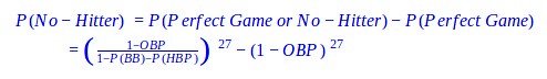
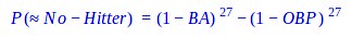
(This is Part 4 of a four-part series answering common questions regarding starting pitchers by use of discrete probability models. In Part 1 we explored perfect game and no-hitter probabilities, in Part 2 we further investigated other hit probabilities in a complete game, and in Part 3 we predicted the winner of pitchers’ duels. Here we project the probability of scoring at least one run in various base runner and out scenarios.)

V.  I Don’t Know’s on Third!

Still far from a distant memory, the final out of the 2014 World Series was preceded by an unexpected single and a nerve-racking error that brought Alex Gordon to 3^rd base with two outs. Closer Madison Bumgarner, who was on fire throughout the playoffs as a starter, allowed the hit but would be left in the game to finish the job. There is some debate as to whether Gordon should have been sent home rather than stopped at 3^rd base , but it would have taken another error overshadowing Bill Buckner’s to get him home; also, next up to bat was Salvador Perez, the only player to ever ding a run off Bumgarner in three World Series. So even though the Royals’ 3^rd Base Coach Mike Jirschele had to make a spur of the moment critical decision to stop Gordon as he approached 3^rd base, it was a decision validated by both statistics and common sense. We will show our own evidence, by use of negative multinomial probabilities, of how unlikely the Royals would have scored the tying run off of Bumgarner with a runner on 3^rd with two outs and we will also consider other potential game-tying or winning situations.

Runs are generally strung together from sequences of hits, walks, and outs; in the situations we will consider, we will only focus on those sequences that lead to at least one run scoring and those that do not. Events not controlled by the batter in the box, such as steals and errors, could also potentially reshape the situation and lead to runs, but we’ll take a very conservative approach and assume a cautious situation where steals are discouraged and errors are extremely unlikely.

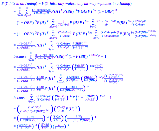
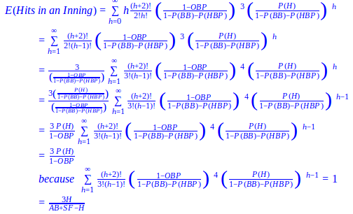
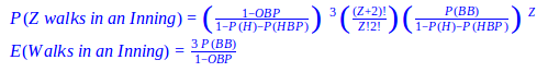
Let A and B be random variables for hits and walks and let P(H) and P(BB) be their respective probabilities for a specific pitcher, such that OBP = P(H) + P(BB) + P(HBP) and (1-OBP) is the probability of an out; we combine the hit-by-pitch probability into the walk probability, such that P(BB) is really P(BB) + P(HBP) because we excluded hit-by-pitches from our models, P(HBP) > 0 against Bumgarner in the 2014 World Series, and the result on the base paths is the same as a walk. The first negative multinomial probability formula we’ll introduce considers the sequences of hits, walks, and an out that can occur after two outs have been accumulated, setting the hypothetical stage for the last play in Game 7 of the 2014 World Series.

In the 2014 World Series, Bumgarner’s dominantly low P(H) and P(BB) were respectively 0.123 and 0.027 and his (1-OBP) was 0.849; by applying these values to the formula above we can generate the probabilities of various hit and walk combinations shown in Table 5.1. The yellow highlighted cells in the table represent the combination of hits and walks that would let Bumgarner escape the inning without allowing the tying run (given a runner on 3^rd with two outs and a one run lead). By combining these yellow cells, we see that the odds were overwhelmingly in in Bumgarner’s favor (0.873); all he had to do was get Perez out, walk Perez and get the next batter out, or walk two batters and get the third out.

Table 5.1: Probability of Hit and Walk Combinations after 2 Outs

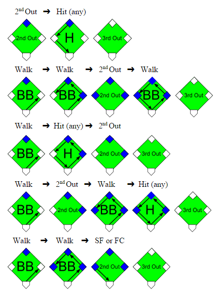
The Royals could have contrarily tied the game with a simple hit from Perez given the runner on 3^rd and two outs, yet this wasn’t the only sequence that would have kept the Royals hopes alive. Three consecutive walks, one walk and one hit, or any combination of walks and one hit could have also done the job; examples of these sequences are shown in the graphics below:

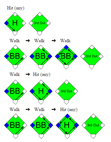
Generally, any combination of walks and hits not highlighted yellow in Table 5.1 would have tied or won the World Series for the Royals. This glimmer of hope was a quantifiable 0.127 probability for Kansas City, so it was justified that Gordon was kept at 3^rd rather than sent home after shortstop Brandon Crawford just received the ball. It would have taken an error from Crawford or Buster Posey, with respective 0.033 and 0.006 2014 error rates, to get Gordon home safely. The probability 0.127 of winning the game from the batter’s box is noticeably three times greater than the probability of winning it from the base paths (where Crawford and Posey’s joint error probability was 0.039).

We should note that the layout in Table 5.1 is a simplification of what could occur with a runner on 3^rd, two outs, and a one run lead, because it only applies to innings where a walk off is not possible. In innings where a walkoff can occur, such as the bottom of the 9th, the combinations of walks and hits captured in the red highlighted cells are not possible because they would occur after the winning run has scored and the game has ended. However, Bumgarner was so dominant in the World Series that these probabilities are almost non-existent, thereby making our model is still applicable; we would otherwise exclude these red-celled probabilities for less successful pitchers.

The next probability formula considers the sequences of walks, hits, and outs that can occur after one out has been accumulated, which is situation definitely worth examining if there is a lone runner on 2^nd base.

Once again we’ll use Bumgarner’s 2014 World Series statistics to evaluate this formula and insert the probabilities into Table 5.2. According to the sum of the yellow cells, Bumgarner would be able to prevent the tying run from scoring (from 2^nd base with one out) with a probability of 0.762 and would otherwise allow the tying run with a probability of 0.238.

Table 5.2: Probability of Hit and Walk Combinations after 1 Out

To get out of the inning unscathed, Bumgarner would need to prevent any further hits or allow fewer than 3 walks given a runner on 2^nd with 1 out; it would be possible to advance the runner to on 3^rd with 2 walks and then sacrifice him home in this situation (with no hits), but this probability is insignificantly tiny especially for a dominant pitcher like Bumgarner. Once again we depict these sequences that could get the tying run home from 2^nd with 1 out, with the second out inserted randomly.

A runner on 2^nd base with one out is a scenario commonly manufactured in an attempt to tie the game from a runner on 1^st with no outs situation. The logic is that if the hitting team is down by one run and the first batter leads off the inning with a single or walk, the next batter can control getting him into scoring position and hope that either of the next two batters knocks the run in with a hit. However, this method of control, a bunt, sacrifices an out to move the runner from 1^st to 2^nd. The defense will usually allow the hitting team to move the runner into scoring position for an out, but the out wasn’t the only sacrifice made. The inning is truncated for the hitting team with one less batter and the potential to have more hitters bat and drive in runs is reduced. Indeed, against a pitcher like Bumgarner, the out is likely not worth the meager 0.238 probability of getting that runner home.  We’ll see in the next section what exactly gets sacrificed for this chance at tying the game.

We should note that in this “runner on 2^nd with 1 out” model we added few more assumptions to those we made in the prior “runner on 3^rd with 2 outs” model, neither of which should be farfetched. The first assumption is that with the game close and the manager intent on tying the game rather than piling on runs, he should have a runner on 2^nd base fast enough to score on a single. Another assumption is that the base runners will be precautious enough not to cause an out on the base paths, yet aggressive enough not to get doubled up or have the lead runner sacrificed in a fielder’s choice play. Lastly, we assume that the combinations of hits, walks, and outs are random, even though we know the current state of base runners and outs can have a predictive effect on the next outcome and the defensive strategy used. By using these assumptions we simplify the factors and outcomes accounted for in these models and reduce the variability between each model.

The final probability formula considers the sequences of walks, hits, and outs that can occur when we start with no outs accumulated; this allows to forge situation will allow us to forge the outcomes from a runner on 1^st with no outs scenario and compare them to a runner on 2^nd with 1 out scenario.

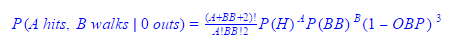
Table 5.3 below uses Bumgarner’s 2014 World Series statistics, the same as before, although in this model we deal with more uncertainty because the sequences captured in each box are not as clear cut between run scoring or not given a runner on 1^st with no outs. The yellow and non-highlighted cells are still the respective probabilities of not allowing and allowing the tying run to score, however, we now introduce the green probabilities to represent the hit and walk combinations that could potentially score a run but are dependent on the hit types, sequences of events, and the use of productive outs. These factors were unnecessary in the prior two models because in those models any hit would have scored the run, the sequence of events was inconsequential, and the use of productive outs was unnecessary with the runner is already on 2^nd or 3^rd base (except when there is a runner on 3^rd and a sacrifice fly or fielder’s choice could bring him home).

Table 5.3: Probability of Hit and Walk Combinations after 0 Outs

We must break down each green probability into subsets of yellow probabilities representing the specific sequences that would not score the tying run from 1^st base with no outs; we depict these sequences below, but for simplicity, not all are depicted.

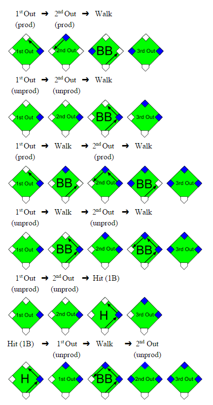
Now that we know the conditions when a run would not score, we take the probabilities from the green cells in Table 5.3, narrow them down according to the proportion of sequences and the proportion of hit types that would not score the run, and separate them based on the usage of productive and unproductive outs; the results are displayed in Table 5.4. For example, there are 6 possible combinations for 1 hit, 1 walk, and 3 outs and 3 of these 6 combinations would not score the tying run on a single, where P(1B | H) = 0.755, with unproductive outs; yet, the run would score with productive outs, with unproductive outs on a double or better, or with unproductive outs and the other 3 combinations. When we finally sum these yellow cells, they tell us that an aggressive manager would score the tying run against Bumgarner with a 0.370 probability and Bumgarner would escape the inning with a 0.630 probability. Otherwise, a less aggressive manager would score the tying run with a mere 0.154 probability and Bumgarner would leave unscathed with a significant 0.846 probability.

Table 5.4: Probability of No Runs Scoring after 0 Outs

We summarize the results from Tables 5.1-5.4 into Table 5.5 from the perspective of the hitting team.  We compare their chances of success not only against Madison Bumgarner from the 2014 World Series but also against Tim Lincecum, Matt Cain, and Jonathan Sanchez from the 2010 World Series.

Table 5.5: Probability of Allowing at least One Run to Score

Let’s return to the scenario that is the launching point for this study… The hitting team is down by one run and there is a runner on 1^st base with no outs. If the game is in its early innings, where it is not mandatory that this runner at 1^st gets home, the manager will likely decide against being aggressive and avoid sacrificing outs in order to increase his chances of extending the inning to score more runs; there are several studies supporting this logic. Yet, if the game is in the latter innings and base runners are hard to come by, the manager should lean towards utilizing productive outs and intentionally sacrifice the runner from 1^st to 2^nd base. His shortsighted goal should only be to tie the game.  By forcing productive outs rather than being conservative on the base paths, his chances of tying the game increase significantly (between 0.216 and 0.271) against our four pitchers given a runner on 1^st and no outs scenario.

However, the if the manager does successfully orchestrate the runner from 1^st to 2^nd base with a productive out, he does still lose a little bit of probability of tying the game; between 0.132 and 0.215 of probability is lost against our pitchers. And if he decides to sacrifice the runner further from 2^nd to 3^rd base with another out, his team’s chances would decrease again by a comparable amount; this decision is ill-advised because a hit is likely going to be needed to tie the game and the hitting team would be sacrificing one of two guaranteed chances to hit in this situation. In general, the probability of scoring at least one run decreases as more outs are accumulated, regardless of the base runners advancing with each out. The manager could contrarily decide against sacrificing his batter if he has confidence that his batter can hit the pitcher or draw a walk, yet the imperative goal is still to tie the game. The odds of tying the game actually favor an aggressive hitting team that is able to get the runner to 2^nd base with one out, by an improvement ranging from 0.012 to 0.084, over a less aggressive team with a runner at 1^st with no outs. Thus, even though sacrificing the runner from 1^st to 2^nd base does decrease the chances of tying the game, it would be worse to approach the game lifelessly when the situation demands otherwise.

(This is Part 3 of a four-part series answering common questions regarding starting pitchers by use of discrete probability models. In Part 1 we explored perfect game and no-hitter probabilities and in Part 2 we further investigated other hit probabilities in a complete game. Here we project the probability of winning a pitchers’ duel for who will allow the first hit.)

IV. Pitchers’ Duels

Bronze statues and folk songs are created to honor legendary feats of strength and stoicism… And Madison Bumgarner is deserving given his performance in the 2014 World Series. On baseball’s biggest stage, Bumgarner not only steamrolled an undefeated Royals team that was firing on all cylinders but he also posted timeless statistics (21 IP, 0.43 ERA, 0.127 BAA) that were beyond Ruthian or Koufaxian. Even as a rookie hidden among the 2010 Giants World Series rotation, Bumgarner’s potential radiated. So what do you do with an athlete who transcends time? You throw him into hypothetical matchups versus other champions. It would be thrilling, unless you like runs, to pit him against a pack of no-hitter-throwing pitchers (his 2010 rotation-mates) and even his 2010 self. We would be treated to great pitchers’ duels comparable to the matchups we would expect from a World Series.

When you oppose an excellent starting pitcher against another (and their hitters), the results will likely not reflect each players’ season averages. Hits and walks will be hard to come by and runs will be even harder. For our duels, we use each pitcher’s World Series probability of a hit, P(H), Bumgarner from 2014 and 2010 and the rest from 2010; P(H), hits divided by the same base as on-base percentage (AB+SF+HBP+BB), represents the quality of pitching we want from our duels. Even though 2014 Bumgarner faced a different lineup (the Royals) than the lineup his 2010 rotation-mates faced (the Rangers) to produce their respective averages, we are encapsulating the performances witnessed and assuming they can be recreated for our matchups. If okay with this assumption, then we can construct a probability model that predicts which pitcher will allow the first hit in our hypothetical pitchers’ duels. If interested further, we could also switch the variables to predict which pitcher will allow the first base runner by using on-base percentage (OBP).

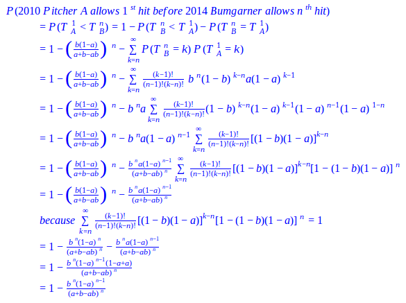
The first formula we construct determines the probability that 2010 Pitcher A will allow m hits before 2014 Bumgarner allows his 1^st hit; it is possible for the m^th hit from A and the 1^st hit from Bumgarner to occur after the same number of batters, but in a duel we want a clear winner. Let a be P(H) for 2010 Pitcher A and be a random variable for the total batters faced when he allows his m^th hit; similarly, let b be P(H) for 2014 Bumgarner and be a random variable for the total batters faced when he allows his 1^st hit. If 2010 Pitcher A allows his m^th hit on the j^th batter, he will have a combination of m hits and (j-m) non-hits (outs, walks, sacrifice flies, hit-by-pitches) with the respective probabilities of a and (1-a); meanwhile 2014 Bumgarner will eventually allow his 1^st hit on the (j+1)^th batter or later and he will have 1 hit and the rest non-hits with the respective probabilities of b and (1-b). We can then sum each j^th scenario together for any number of potential batters faced (all j≥m) to create the formula below:

If we assume an even pitchers’ duel of who will allow the 1^st hit, for m=1, then we have the following intuitive formula for 2010 Pitcher A versus 2014 Bumgarner:

This formula takes the probability that 2010 Pitcher A allows a hit minus the probability that both pitchers allow a hit and divides it by the probability that 2010 Pitcher A or 2014 Bumgarner allow a hit. Furthermore, if we let this happen for m hits, we arrive at our deduced formula. We should also note that according to the deduced formula, we should see the probability decrease as m increases. This logic makes sense because the expected span of batters until 2014 Bumgarner allows his 1^st hit, , stays the same, but we are trying to squeeze in more hits allowed by 2010 Pitcher A, which makes the probability become less likely.

Table 4.1:  Probability of 2010 Pitcher A Allowing m^th Hit Before 2014 Bumgarner Allows 1^st

In Table 4.1, we compare 2014 Bumgarner and his 0.123 World Series P(H) versus each starter from the 2010 World Series Giants rotation and their respective P(H). We expect 2014 Bumgarner to have the advantage over 2010 Lincecum, Cain, and Sanchez, given how he dominated the 2014 World Series; clearly he does. In an even pitchers’ duel, he would win with a probability greater than 50% even after the chance of a tie is removed; we could even see 2 hits from the other pitchers before 2014 Bumgarner allows his 1^st with a probability greater than 25%. However, against a comparably excellent pitcher, himself in 2010, he would likely lose the duel because 2010 Bumgarner actually has a better P(H). Notice that from Sanchez to Lincecum and from Lincecum to Cain, the P(H) descends steadily each time; consequently, the same pattern of linear decline also follows duel probabilities when transitioning from pitcher to pitcher for each of the different hits allowed. Hence, the distinction between exceptional and below-average pitchers stays relatively constant as we allow more hits by them versus 2014 Bumgarner.

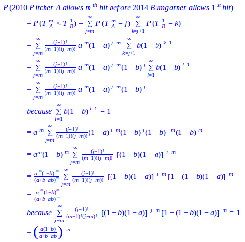
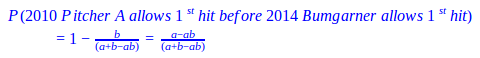
We can also construct the converse formula to calculate the probability that 2010 Pitcher A allows 1 hit before 2014 Bumgarner allows his n^th hit. We let be a random variable for the total batters faced when 2014 Bumgarner allows his n^th hit and for when 2010 Pitcher A allows his 1^st hit. However, instead of directly deducing the probability that 2010 Pitcher A allows 1 hit before 2014 Bumgarner allows his n^th hit, we’ll do so indirectly by taking the complement of both the probability that 2014 Bumgarner allows his n^th hit before 2010 Pitcher A allows his 1^st hit (a variation of our first formula) and the probability that 2014 Bumgarner allows his n^th hit and 2010 Pitcher A allows his 1^st hit after the same number of batters.

The resulting formula takes the complement of the probability that 2014 Bumgarner allows n hits and 2010 Pitcher A does not allow a hit in (n-1) chances and divides it by the probability that 2010 Pitcher A or 2014 Bumgarner allow n hits. In this formula we can contrarily see the probability increase as n increases. By extending the expected span of batters, , to accommodate 2014 Bumgarner’s n hits instead of just 1, we’re granting 2010 Pitcher A more time to allow his 1^st hit, resulting in an increased likelihood.

Once again, if we set n=1 for an even matchup, we get the same formula as before:

Table 4.2:  Probability of 2010 Pitcher A Allowing 1^st Hit Before 2014 Bumgarner Allows n^th

In Table 4.2, we again use 2014 Bumgarner’s 0.123 P(H) versus those displayed in the table above. As expected, the probabilities from the even duels are the same as Table 4.1 because the formulas are the same. Although this time from Sanchez to Lincecum and from Lincecum to Cain, the difference between each pitcher noticeably decreases as we adjust the scenario to allow 2014 Bumgarner more hits. Thereby, there is less distinction between exceptional and below-average pitchers if we widen the range of batters, , enough for them to allow their 1^st hit versus 2014 Bumgarner.

Madison Bumgarner may have dominated the 2014 World Series as a starter, but he also forcefully shut the door on the Royals to carry his team to the title (by ominously throwing 5 IP, 2 H, 0 BB). Given the momentum he had, he proved himself to be Bruce Bochy’s best option. However, not every game is Game 7 of the World Series, where a manager must decisively bring in the one reliever he trusts the most. A manager needs to assess who is the appropriate reliever for the job and weigh which relievers will available later. Fortunately, an indirect benefit of the pitchers’ duel model is that it can calculate the relative probability between two relievers for who will allow a hit or baserunner first; this application could be very useful in long relief or in extra innings.

Table 4.3:  Probability of 2010 Pitcher A Allowing m^th Baserunners Before 2014 Bumgarner Allows 1^st

Suppose we’re entering extra innings and the only pitchers available are 2014 Bumgarner and 2010 Bumgarner, Lincecum, Cain, and Sanchez with their respective statistics from Table 4.3 (where we substituted P(H) in Table 4.1 for OBP). We wouldn’t automatically throw in our best pitcher, 2014 Bumgarner, with his 0.151 OBP; we need to compare how he would perform relative to the other 2010 pitchers and see what the drop off is. Nor is it a priority to know how many innings to expect out of our reliever because we don’t know how long he’ll be needed. What is crucial in this situation is the prevention of baserunners as potential runs. 2010 Bumgarner, Cain, and Lincecum would each be worthy candidates to keep 2014 Bumgarner in the bullpen, because each has a reasonable chance (greater than 40%) of allowing a baserunner by the same batter or later than 2014 Bumgarner. Hence, the risk of using a pitcher with a slightly greater chance of allowing a baserunner sooner may be worth the reward of having 2014 Bumgarner available in a more dire situation. Yet, we would want to avoid bringing in 2010 Sanchez because the risk would be too great; the probability is approximately 49% that he could allow two baserunners before 2014 Bumgarner allows one. Preventing baserunners and using your bullpen appropriately are both high priorities in close game situations where mistakes are magnified.

(This is Part 2 of a four-part series answering common questions regarding starting pitchers by use of discrete probability models.  In Part 1, we dealt with the probability of a perfect game or a no-hitter. Here we deal with the other hit probabilities in a complete game.)

III. Yes! Yes! Yes, Hitters!

Rare game achievements, like a no-hitter, will get a starting pitcher into the record books, but the respect and lucrative contracts are only awarded to starting pitchers who can pitch successfully and consistently. Matt Cain and Madison Bumgarner have had this consistent success and both received contracts that carry the weight of how we expect each pitcher to be hit. Yet, some pitchers are hit more often than others and some are hit harder. Jonathan Sanchez had shown moments of brilliance but pitch control and success were not sustainable for him. Tim Lincecum had proven himself an elite pitcher early in his career, with two Cy Young awards, but he never cashed in on a long term contract before his stuff started to tail off. Yet, regardless of success or failure, we can confidently assume that any pitcher in this rotation or any other will allow a hit when he takes the mound. Hence, we should construct our expectations for a starting pitcher based on how we expect each to get hit.

An inning is a good point to begin dissecting our expectations for each starting pitcher because the game is partitioned by innings and each inning resets. During these independent innings a pitcher’s job is generally to keep the runners off the base paths. We consider him successful if he can consistently produces 1-2-3 innings and we should be concerned if he alternately produces innings with an inordinate number of base runners; whether or not the base runners score is a different issue.

Let BR be the base runners we expect in an inning and let OBP be the on-base percentage for a specific starting pitcher, then we can construct the following negative binomial distribution to determine the probabilities of various inning scenarios:

If we let br be a random variable for base runners in an inning, we can apply the formula above to deduce how many base runners per inning we should expect from our starting pitcher:

The resulting expectation creates a baseline for our pitcher’s performance by inning and allows us to determine if our starting pitcher generally meets or fails our expectations as the game progresses.

Table 3.1: Inning Base Runner Probabilities by Pitcher

Based upon career OBPs through the 2013 season, Bumgarner would have the greatest chance (0.356) of retiring the side in order and he would be expected to allow the fewest base runners, 1.233, in an inning; Cain should also have comparable results. The implications are that Bumgarner and Cain represent a top tier of starting pitchers who are more likely to allow 0 base runners than either 1 base runner or +2 base runners in an inning. A pitcher like Lincecum, expected to allow 1.326 base runners in an inning, represents another tier who would be expected to pitch in the windup (for an entire inning) in approximately ⅓ of innings and pitch from the stretch in ⅔ of innings. Sanchez, on the other hand, represents a respectively lower tier of starting pitchers who are more likely to allow 1 or +2 base runners than 0 base runners in an inning. He has the least chance (0.280) of having a 1-2-3 inning and would be expected to allow more base runners, 1.586, in an inning.

As important as base runners are for turning into runs, the hits and walks that make up the majority of base runners are two disparate skills.  Hits generally result from pitches in the strike zone and demonstrate an ability to locate pitches, contrarily, walks result from pitches outside the strike zone and show a lack of command.  Hence, we’ll create an expectation for hits and another for walks for our starting pitchers to determine if they are generally good at preventing hits and walks or prone to allowing them in an inning.

Let h, bb, and hbp be random variables for hits, walks, and hit-by-pitches and let P(H), P(BB), P(HBP) be their respective probabilities for a specific starting pitcher, such that OBP = P(H) + P(BB) + P(HBP). The probability of Y hits occurring in an inning for a specific pitcher can be constructed from the following negative multinomial distribution:

We can further apply the probability distribution above to create an expectation of hits per inning for our starting pitcher:

For walks, we do not have to repeat these machinations.  If we simply substitute hits for walks, the probability of Z walks occurring in an inning and the expectation for walks per inning for a specific pitcher become similar to the ones we deduced earlier for hits:

We could repeat the same substitution for hit-by-pitches, but the corresponding probability distribution and expectation are not significant.

Table 3.2: Inning Hit Probabilities by Pitcher

The results of Table 3.2 and Table 3.3 are generated through our formulas using career player statistics through 2013. Cain has the highest probability (0.466) of not allowing a hit in an inning while Sanchez has the lowest probability (0.439) among our starters. However, the actual variation between our pitchers is fairly minimal for each of these hit probabilities. This lack of variation is further reaffirmed by the comparable expectations of hits per inning; each pitcher would be expected to allow approximately 0.9 hits per inning. Yet, we shouldn’t expect the overall population of MLB pitchers to allow hits this consistently; our the results only indicate that this particular Giants rotation had a similar consistency in preventing the ball from being hit squarely.

Table 3.3: Inning Walk Probabilities by Pitcher

The disparity between our starting pitchers becomes noticeable when we look at the variation among their walk probabilities. Bumgarner has the highest probability (0.776) of getting through an inning without walking a batter and he has the lowest expected walks (0.264) in an inning. Sanchez contrarily has the lowest probability (0.589) of having a 0 walk inning and has more than double the walk expectation (0.580) of Bumgarner. Hence, this Giants rotation had differing abilities targeting balls outside the strike zone or getting hitters to swing at balls outside the strike zone.

Now that we understand how a pitcher’s performance can vary from inning to inning, we can piece these innings together to form a 9 inning complete game. The 9 innings provides complete depiction of our starting pitcher’s performance because they afford him an inning or two to underperform and the batters he faces each inning vary as he goes through the lineup. At the end of a game our eyes still to gravitate to the hits in the box score when evaluating a starting pitcher’s performance.

Let D, E, and F be the respective hits, walks, and hit-by-pitches we expect to occur in a game, then the following negative multinomial distribution represents the probability of this specific 9 inning game occurring:

Utilizing the formula above we previously answered, “What is the probability of a no-hitter?”, but we can also use it to answer a more generalized question, “What is the probability of a complete game Y hitter?”, where Y is a random variable for hits. This new formula will not only tell us the probability of a no-hitter (inclusive of a perfect game), but it will also reveal the probability of a one-hitter, three-hitter, etc. Furthermore, we can calculate the probability of allowing Y hits or less or determine the expected hits in a complete game.

Let h, bb, hbp again be random variables for hits, walks, and hit-by-pitches.

The derivations of the complete game formulas above are very similar to their inning counterparts we deduced earlier. We only changed the number of outs from 3 (an inning) to 27 (a complete game), so we did not need to reiterate the entire proofs from earlier; these formulas could also be constructed for an 8 inning (24 outs), a 10 2/3 inning (32 outs), or any other performance with the same logic.

Table 3.4: Complete Game Hit Probabilities by Pitcher using BA

The results of Table 3.4 were generated from the complete game approximation probabilities that use batting average (against) as an input. Any of the four pitchers from the Giants rotation would be expected to allow 8 or 9 hits in a complete game (or potentially 40 total batters such that 40 = 27 outs + 9 hits + 4 walks), but in reality, if any of them are going to be given a chance to throw a complete game they’ll need to pitch better than that and average less than 3 pitches per batter for their manager to consider the possibility. If we instead establish a limit of 3 hits or less to be eligible for a complete game, regardless of pitch total, walks, or game situation (not realistic), we could witness a complete game in at most 1 or 2 starts per season for a healthy and consistent starting pitcher (approximately 30 starts with a 5% probability). Of course, we would leave open the possibility for our starting pitcher to exceed our expectations by throwing a two-hitter, one-hitter, or even a no-hitter despite the likelihood. There is still a chance! Managers definitely need to know what to expect from their pitchers and should keep these expectations grounded, but it is not impossible for a rare optimal outcome to come within reach.

I. Introduction

In the statistics driven sport of baseball, the fans who once enjoyed recording each game in their scorecard have become less accepting of what they observe and now seek to validate each observation with statistics.  If the current statistics cannot support these observations, then they will seek new and authenticated statistics.

The following sections contain formulas for statistics I have not encountered, yet piqued my curiosity, regarding the 2010 Giants’ World Series starting rotation.  Built around Tim Lincecum, Matt Cain, Jonathan Sanchez, and Madison Bumgarner, the 2010 Giants’ strength was indeed starting pitching.  Each player was picked from the Giants farm system, three of them would throw a no-hitter (or perfecto) as a Giant, and of course they were the 2010 World Series champions.  Throw in a pair of Cy Young awards (Lincecum), another championship two years later (Cain, Bumgarner, Lincecum), eight all-star appearances between them (Cain, Bumgarner, Lincecum), and this rotation is highly decorated.  But were they an elite rotation?

II. Perfectos & No-No’s

It certainly seems rare to have a trio of no-hit pitchers on the same team, let alone home-grown and on the same championship team.  No-hitters and perfect games factor in the tangible (a pitcher’s ability to get a batter out and the range of the defense behind him) and the intangible (the fortitude to not buckle with each accumulated out).  Tim Lincecum, Matt Cain, and Jonathan Sanchez each accomplished this feat before reaching 217th career starts, but how many starts would we have expected from each pitcher to throw a no-hitter or perfect game?  What is the probability of a no-hitter or perfect game for each pitcher?  We definitely need to savor these rare feats.  Based on the history of starting pitchers with career multiple no-hitters, it is unlikely that any of them will throw a no-hitter or perfect game again.  Nevermind, it happened again for Lincecum a few days ago.

First we deduce the probability of a perfect game from the probability of 27 consecutive outs:

Table 2.1: Perfect Game Probabilities by Pitcher

The probability of a perfect game is calculated for each pitcher (above) using their exact career on-base percentage (OBP rounded to three digits) through the 2013 season.  Based on these calculations, we would expect 1 in 12,152 of Matt Cains starts to be perfect.  Although it didn’t take 12,152 starts to reach this plateau, he achieved his perfecto by his 216th start.  For Tim Lincecum, we would expect 1 in 19,622 starts to be perfect; but starting even 800 starts in a career is very farfetched.   Durable pitchers like Roger Clemens and Greg Maddux only started as many as 707 and 740 games respectively in their careers and neither threw a perfect game nor a no-hitter.  No matter how elite or if Hall of Fame bound, throwing a perfect game for any starting pitcher is very unlikely and never guaranteed.  However, that infinitesimal chance does exist.  The probability that Jonathan Sanchez would throw a perfect game is a barely existent chance of 1 in 94,488, but he was one error away from a throwing a perfect game during his no-hitter.

The structure of a no-hitter is very similar to a perfect game with the requirement of 27 outs, but we include the possibility of bb walks and hbp hit-by-pitches (where bb+hbp≥1) randomly interspersed between these outs (with the 27th out the last occurrence of the game).  We exclude the chance of an error because it is not directly attributed to any ability of the pitcher.  In total, a starting pitcher will face 27+bb+hbp batters in a no-hitter.  Using these guidelines, the probability of a no-hitter can be constructed into a calculable formula based on a starting pitcher’s on-base percentage, the probability of a walk, and the probability of a hit-by-pitch.  Later we will see that this probability can be reduced into a simpler and more intuitive formula.

Let h, bb, hbp be random variables for hits, walks, and hit-by-pitches and let P(H), P(BB), P(HBP) be their respective probabilities for a specific starting pitcher, such that OBP = P(H) + P(BB) + P(HBP).  The probability of a no-hitter or perfect game for a specific pitcher can be constructed from the following negative multinomial distribution (with proof included):

This formula easily reduces to the probability of a no-hitter by subtracting the probability of a perfect game:

The no-hitter probability may not be immediately intuitive, but we just need to make sense of the derived formula. Let’s first deconstruct what we do know… The no-hitter or perfect game probability is built from 27 consecutive “events” similar to how the perfect game probability is built from 27 consecutive outs.  These “event” and out probabilities can both broken down into a more rudimentary formulas. The out probability has the following basic derivation:

The “event” probability shares a comparable derivation that utilizes the derived out probability and the assumption that sacrifice flies are usually negligible per starting pitcher per season:

From this breakdown it becomes clear that the no-hitter (or perfect game) probability is logically constructed from 27 consecutive at bats that do not result in a hit, whose frequency we can calculate by using the batting average (BA). Recall that a walk, hit-by-pitch, or sacrifice fly does not count as an at bat, so we only need to account for hits in the no-hitter or perfect game probability. Hence, the batting average in conjunction with the on-base percentage, which does include walks and hit-by-pitches, will provide an accurate approximation of our original no-hitter probability:

Comparing the approximate no-hitter probabilities to their respective exact no-hitter probabilities in Table 2.2, we see that these approximations are indeed in the same ball park as their exact counterparts.

Table 2.2: No-Hitter Probabilities by Pitcher

The probability of a no-hitter is calculated for each pitcher (above) using their exact career on-base percentage, walk probability, and hit-by-pitch probability through the 2013 season.  Notice that the likelihood of throwing a no-no is significantly greater than that of a perfecto for each pitcher.  For example, Lincecum and Cain’s chances of making no-no history are far easier than being perfect by the respective factors of 15.9 and 11.5.  Although Lincecum and Cain are still both unlikely to accumulate the 1,231 and 1,055 starts necessary to ascertain these no-hitter probabilities.  If it’s any consolation, Lincecum already achieved his no-hitter by his 207th start (and another by his 236th start) and Cain already has a perfecto instead.

Furthermore, it’s possible for two pitchers with disparate perfect game probabilities to have very similar no-hitter probabilities, as we see with Sanchez and Bumgarner.  Sanchez has a no-hitter probability of 1 in 1,681 that is 56.2 times greater than his perfect game probability, while Bumgarner’s 1 in 1,772 probability is a mere 6.1 times greater.  This discrepancy can be attributed to Sanchez’ improved ability to not induce hits versus his tendency to walk batters, while Bumgarner’s improvement is of a lesser degree.  Regardless, Sanchez’ early no-hitter, achieved by his 54th start, can instill hope in Bumgarner to also beat the odds and join his 2010 rotation mates in the perfect game or no-hitter’s club.  Adding Bumgarner to the brotherhood would greatly support the claim that the Giants 2010 starting rotation was extraordinary.  However, the odds still fall in my favor that I will not need to rewrite this section of this study due to another unexpected no-no or perfecto by Lincecum, Cain, Sanchez, or Bumgarner.

I. Introduction

A starting pitcher should have the advantage over opposing batters throughout a baseball game, yet as he pitches further into the game this advantage should slowly decrease.  The opposing manager hopes that his batters can pounce on the wilting starting pitcher before his manager removes him from the game.  But what would we see if the manager decided against removing his starting pitcher?  The goal of this analysis is to determine the consequences of allowing an average starting pitcher to pitch further into the game instead of removing him.  There are several different ways this situation can unfold for a starting pitcher, but we should be able to tether our expectations to that of an average starting pitcher.

We will focus on how the total pitches thrown by starting pitchers (per game) affects runs, outs, hits, walks, strikes, and balls by analyzing their corresponding probability distributions (Figures 1.1-1.6) per pitch count; the x-axis represents the pitch count and the y-axis is the probability of the chosen outcome on the i^th pitch thrown.  Each plot has three distinct sections:  Section 3 is where the uncertainty from the decreasing pitcher sample sizes exceeds our desired margin of error (so we bound it with a confidence interval); Section 1 contains the distinct adjustment trend for each outcome that precedes the point where the pitcher has settled into his performance; Section 2, stable relative to the others sections, is where we hope to find a generalized performance trend with respect to the pitch count for each outcome.  Together these sections form a baseline for what to expect from an average starting pitcher.  Managers can then hypothesize if their own starting pitcher would fare better or worse than the average starting pitcher and make the appropriate decisions.

II.  Data

From 2000-2004, 12,138 MLB games were played; there should have been 12,150 games but 12 games were postponed and never made up.  During this period, starting pitchers averaged 95.12 pitches per game with a standard deviation of 18.21.  The distribution of pitch counts is normal with a left tail that extends below 50 pitches (Figure 2).  It is not symmetric about the mean because a pitcher is more likely to be inefficient or injured early (left tail) than to exceed 150 pitches.  In fact, no pitcher risked matching Ron Villone’s 150 pitch count from the 2000 season.

This brief period was important for baseball because it preceded a significant increase in pitch count awareness.  From 2000-2004, there averaged 192 pitching performances ≥122 pitches per season (Table 2); 122 is the sampling threshold explained in the next section.  Since then, the 2005-2009 seasons have averaged only 60 performances ≥122 pitches per season.  This significant drop reveals how vital pitch counts have become to protecting the pitcher and controlling the outcome of the game.  Now managers more frequently monitor their pitchers’ and the opposing pitchers’ pitch counts to determine when they will expire.

Table 2:  2000-2009 Starting Pitcher Pitch Counts ≥122

III. Sampling Threshold (Section 3)

122 pitches is the sampling threshold deduced from the 2000-2004 seasons (and the pitch count minimum established for Section 3), but it is not necessarily a pitch count threshold of when to pull the starting pitcher.  Instead this is the point when starting pitcher data becomes unreliable due to sample size limitations.  Beyond 122 pitches, the probabilities of Figures 1.1-1.6 violently waver high and low as very few pitchers threw more than 122 pitches.  A smoothed trend, represented by a dashed blue line and bounded by a 95% confidence interval was added to Section 3 of Figures 1.1-1.6 to contain the general trend between these rapid fluctuations.  But the margin of error (the gap between the confidence interval and the smoothed trend) grows exponentially beyond 3%, so the actual trend could be anywhere within this margin.  Thereby, we cannot hypothesize whether it is more or less likely that the pitcher’s performance will excel or plummet after 122 pitches.

To understand how the 122 sampling threshold was determined, we first extract the margin of error formula (e) from the confidence interval formula (where  z_α/2 = z-value associated with the (1-α/2)^th percentile of the standard normal distribution, S = standard error of the sample population, n = sample size, N = population size):

Next, we back-solve this formula to find the maximum sample size n for when the margin of error exceeds 3%; we use S = 0.5, z_2.5% = 1.96, N = 2 pitchers × 12,138 games = 24,276:

There is no pitch count directly associated with the sample size of 1,022, but 1,022 can be bounded between the 121 (n=1,147) and 122 (n=971) pitch counts.  At 121 pitches the margin of error is still less than 3%, but it becomes greater than 3% at 122 pitches and begins to increase exponentially.  This is the point the sample size becomes unreliable and the outcomes are no longer representative of the population.  Indeed only 4% (971 of 24,276) of the pitching performances from 2000-2004 equaled or exceeded 122 pitches thrown in a game (Figure 3).

A benefit of the sampling threshold is that it separates the outcomes we can make definitive conclusions about (<122 pitches) from those we cannot (≥122 pitches).  If were able to increase the sampling threshold another 10 pitches, we could make conclusions about the throwing up to 131 pitches in a game.  However, managers will neither risk the game outcome nor injury to their pitcher to accurately model their pitcher’s performance at high pitch counts.  Instead, the sampling thresholds have steadily decreased since 2005 and the 2000-2004 period is likely the last time we’ll be able to make generalizations about throwing 121 pitches in a game.

Yet, even for the confident manager, 121 pitches is still a fair point in the game to assess a starting pitcher.  Indeed the starting pitcher must have been consistent and trustworthy to pitch this deep into the game.  But if the manager wants to allow his starting pitcher to continue pitching, he is only guessing that this consistency will follow because there is not enough data to accurately forecast his performance.  Instead he should consider replacing his starting pitcher with a relief pitcher.  The relief pitcher is a fresh arm that offers less risk; he must have a successful record based on an even smaller sample size of appearances, smaller pitch counts, and a smaller margin of error.  The reliever and his short leash are the surer bet than a starting pitcher at 122 pitches.

IV.  Adjustment Period (Section 1)

The purpose of the adjustment period is to allow the starting pitcher a generous period to find a pitching rhythm.  No conclusions are made regarding the probabilities in the adjustment period as long as an inordinate amount of walks, hits, and runs are not allowed.  The most important information we can impart from this period is the point when the adjustment ends.  Once the rhythm is found, we can be critical of a pitcher’s performance and commence the performance trend analysis.

In order to be effective from the start, starting pitchers must quickly settle into an umpire’s strike zone and throw strikes consistently; most pitchers do so by the 3^rd pitch of the game (Figure 1.5).  Consistent strike throwing keeps the pitcher ahead in the count and allows him to utilize the outside of the strike zone rather than continually challenging the batter in the zone.  Conversely, a pitcher must also include (pitches called) balls into his rhythm, starting approximately by the 8^th pitch of the game (Figure 1.6).  Minimal ball usage clouds the difference between strikes and balls for the batter while frequent usage hints at a lack of control by the pitcher.  Strikes and balls furthermore have a predictive effect on the outcomes of outs, hits, runs, and walks:  a favorable count for the batter forces the pitcher to deliver pitches that catch a generous amount of the strike zone while one in favor of the pitcher forces the batter to protectively swing at any pitch in proximity of the strike zone.

On any pitch, regardless of the count, the batter could still hit the ball into play and earn an out or hit.  Yet as long as the pitcher establishes a rhythm for minimizing solid contact by the 4^th pitch of the game (Figure 1.2-1.3), he can decrease the degree of randomness that factors into inducing outs and minimizing hits.  A walk contrarily cannot occur on any pitch because walks are the result of four accumulated balls.  Pitchers should settle into a rhythm of minimizing walks by using minimal ball usage; so when the ball rhythm stabilizes (on the 8^th pitch of the game) the walk rhythm also stabilizes (Figure 1.4).  After each of these rhythms stabilizes, a rhythm can be established for minimizing runs (a string of hits, walks and sacrifices within an inning) by the 12^th pitch of the game (Figure 1.1).  It is possible for home runs or other quick runs to occur earlier, but pitchers who regularly put their team in an early deficit are neither afforded the longevity to pitch more innings nor the confidence to make another start.

V.  Performance Trend (Section 2)

Each of the probability distributions in Figures 1.1-1.6 provides a generalized portrayal of how starting pitchers performed from 2000-2004, but in terms of applicability they do not depict how an average starting pitcher would have performed.  Not all pitchers lasted to the same final pitch (Figure 2).  The better a pitcher performed the longer he should have pitched into the game, so we would expect each successive subset of pitchers (lasting to greater pitch counts) to have been more successful than their preceding supersets.  Thereby, in order to accurately project the performance of an average starting pitcher the probability distributions need to be normalized, by factors along the pitch count, as if no pitchers were removed and the entire population of pitchers remained at each pitch count.

The pitch count adjustment factor (generalized for all pitchers) is a statistic that must be measurable per pitch rather than tracked per at-bat or inning, so we cannot use batting average, on-base percentage, or earned run average.  The statistic should also be distinct for each outcome because a starting pitcher’s ability to efficiently minimize balls, hits, walks, and runs and productively accumulate strikes and outs are skills that vary per pitcher.  Those who are successful in displaying these abilities will be allowed to extend their pitch count and those who are not put themselves in line to be pulled from the game.

We accommodate these basic requirements by initially calculating the average pitches per outcome x, R_x(t), for any pitcher who threw at least t pitches (where PC_t = sum of all pitch counts and x_t = sum of all x for all pitchers whose final pitch was t):

This statistic, composed of a starting pitcher’s final pitch count divided by his cumulative runs allowed (or the other outcome types), distinguishes the pitcher who threw 100 pitches and allowed 2 runs (50 pitches per run) versus the pitcher with 20 pitches and 2 runs (10 pitches per run).  At each pitch count t, we calculate the average for all starting pitchers who threw at least t pitches; we combine their various final pitch counts (all ≥t), their run totals (occurring anytime during their performance), and take a ratio of the two for our average.  At pitch count 1, the average is calculated for all 24,276 starting pitcher performances because they all threw at least one pitch; the population of starting pitchers allowed a run every 32.65 pitches (Table 5.1).  At pitch count 122, the average is calculated for the 971 starting pitcher performances that reached at least 122 pitches; this subset of starting pitchers allowed a run every 57.75 pitches per game.

Table 5.1:  2000-2004 Pitches per Outcome

Starting pitchers will try to maximize the pitches per outcome averages for runs, hits, walks, and balls while minimizing the probabilities of these outcomes, because the pitches per outcome averages and the outcome probabilities have an inverse relationship.  Conversely, starting pitchers will also try to minimize the pitches per outs and strikes while trying to maximize these probabilities for the same reason.  Hence, we must invert the pitches per outcome averages into outcomes per pitch rates, Q_x(t), to be able to create our pitch count adjustment factor, PCA_x(t), that will compare the change between the population of starting pitchers and the subset of starting pitchers remaining at pitch count t:

The ratio of change is calculated for each outcome x at each pitch count t.  The pitch count adjustment factor, PCA_x(t), will scale p_x(t), the original probability of x from the starting pitchers at pitch count t back to the expected probability of x for an average starting pitcher from the entire population of starting pitchers at pitch count t.

The increases to the pitches per run and pitches per hit rates strongly suggest that the 971 starting pitchers remaining at 122 pitches were more efficient at minimizing runs and hits than the overall population of starting pitchers.  The population performed worse than those pitchers remaining at 122 pitches by factors of 176.85% and 131.98% with respect to the runs per pitch and hits per pitch rates (Table 5.2).  Thereby, we would expect the probability of a run to increase from 3.40% to 6.01% and the probability of a hit to increase from 7.21% to 9.51% if we allowed an average starting pitcher from the population of starting pitchers to throw 122 pitches.

Table 5.2:  2000-2004 Average Pitcher Probabilities at 122 Pitches

We apply the pitch count adjustment factors, PCA_x(t), at each pitch count t to each of the original outcome probability distributions (black) to project the average starting pitcher outcome probabilities (green) for Section 2 (Figures 5.1-5.6); the best linear fit trends (dashed black and green lines) are also depicted.  The reintroduction of the removed starting pitchers noticeably worsened the hit, run, and strike probabilities and slightly improved the out probability in the latter pitch counts.  There were no significant changes to ball and walk probabilities.  These are the general effects of not weeding out the less talented pitchers from the latter pitch counts as their performances begin to decline.

Next we quantify our observations by estimating the linear trends of each original and average pitcher series and then compare their slopes (Table 5.3).  The linear trend (where t is still the pitch count) provides a simple approximation of the general trend of Section 2 while the slope of the linear trend estimates the deterioration rate of the pitcher’s ability to control these outcomes.  The original pitcher trends show that the way managers managed pitch counts, their starting pitchers produced relatively stable probability trends as if the pitch count little or no effect on their pitchers; only the out trend changed by more than 1% over 100 pitches (2.00%).  Contrarily, the average pitcher trends increased by more than 2% over 100 pitches for the run, out, hit, and strike trends, indicating a possible correlation between the pitch count and the average pitcher performance; the walk and ball trends were unchanged from the original to the average starting pitcher.

We must also measure these subtle changes between the original and average trends that occur in the latter pitch counts of Figures 5.1-5.6.  There is rapid deterioration in the ability to throw strikes and minimize hits and runs between the original and average starting pitchers as suggested by the changes in slope.  The 368.21% change in the strike slopes clearly indicates that fewer strikes are thrown by the average starting pitcher in the latter pitch counts.  The factors of 222.53% and 1206.13% for the respective hit and run slopes indicate that the average starting pitcher is not only giving up more hits but giving up more big hits (doubles, triples, home runs).  There is a slight improvement in procuring an out (14.45%), but the pitches that were previously strikes became hits more often than outs for the average starting pitcher.  Lastly, the abilities to minimize balls (4.87%) and walks (8.23%) barely changed between pitchers, so control is not generally lost in the latter pitch counts by the average starting pitcher.  Therefore, the average starting pitcher isn’t necessarily pitching worse as the game progresses but the batters may be getting better reads on his pitches.

Table 5.3:  Section 2 Linear Trend

The correlation coefficients also support our assertion that the average starting pitcher became adversely affected by the higher pitch counts, but even the original starting pitcher showed varied signs being affected by the pitch counts.  There were moderate correlations between the pitch count and hit and walks and a very strong correlation between the pitch count and outs.  So even though some batters improved their ability to read an original starting pitcher’s pitches, this improvement was not consistent and the increases to hits and walks were only modest.  Contrarily, the original starting pitcher did become more efficient and consistent at procuring outs as the pitch count increased.   We also found weak correlations between the pitch count and strikes and balls for the original starting pitcher, so strikes and balls were consistently thrown without any noticeable signs of being affected by the pitch count.   However, out of all of our outcomes, the pitch count of the original starting pitcher had the weakest correlation with runs.  Either the original starting pitchers could consistently pitch independent of the pitch count or their managers removed them before the pitch count could factor into their performance; the latter most likely had the greater influence.

It is also worth noting the intertwined patterns displayed in Figures 5.1-5.6 and Table 5.1.  Strikes and balls naturally complement each other, so it should come as no surprise that the Strike Probability Series and Ball Probability Series also complement each other; a peak in once series is a valley in the other and vice-versa.  The simple reason is that strikes and balls are the most frequent and largest of our outcome probabilities – they are used to setup other outcomes and avoid terminating at-bats in one pitch.  However, fewer strikes and balls are thrown in the latter pitch counts as evidenced by the decline in the Strike and Ball Probability Series, which make the at-bats shorter.  Consequently, there are fewer pitches thrown between the outs, hits, and runs, so these other probability series increase.  Hence, the probabilities of outs, hits, and runs become more frequent per pitch as the pitch count increases (further supported by the drop in pitches per strike and ball rates in Table 5.1).

VI.  Conclusions

Context is very important to the applicability of these results, without it we might conjecture that these trends would continue year over year.  Yet, the 2000-2004 seasons were likely the last time we’ll see a subset of pitchers this large pitching into extremely high pitch counts.   Teams are now very cautious about permitting starting pitchers to throw inconsequential innings or complete games, so the recent populations of starting pitchers have shifted away from the higher pitch counts and throw fewer pitches than before.  Yet, these pitch count restrictions should not affect the stability of our original probability trends.  The sampling threshold will indeed lower and the length of stable Section 2 will shorten, but the stability of the current original trends should not compromise.  Capping the night sooner for the starting pitchers only means they are less likely to tire or be read by batters.

We also cannot generalize that these original probability trends would be stable for any starting pitcher.  The probability trends and their stability are only representative of the shrinking subset of starting pitchers before their managers removed them due to performance issues, injury, strategy, etc.  These starting pitchers subsets may appear unaffected by the pitch count, but their managers created this illusion with the well-timed removal of their starting pitchers.  They understand the symptoms indicative of a declining pitcher and only extend the pitch count leash to starting pitchers who have shown current patterns of success.  Removing managers from the equation would result in an increased number of starting pitchers faltering in the latter pitch counts as their pitches are better read by batters.  Likewise, any runners left on base by the starting pitcher, but now the responsibility of a relief pitcher, would have an increased likelihood of scoring if the starting pitchers were not removed as originally planned by their managers.  Starting pitchers do notice these symptoms and may gravitate to finishing another inning, but each additional pitch could potentially damage the score significantly.  Trust in the manager and let him bear the responsibility at these critical points.