A Discrete Pitchers Study – Predicting Hits in Complete Games

(This is Part 2 of a four-part series answering common questions regarding starting pitchers by use of discrete probability models.  In Part 1, we dealt with the probability of a perfect game or a no-hitter. Here we deal with the other hit probabilities in a complete game.)

III. Yes! Yes! Yes, Hitters!

Rare game achievements, like a no-hitter, will get a starting pitcher into the record books, but the respect and lucrative contracts are only awarded to starting pitchers who can pitch successfully and consistently. Matt Cain and Madison Bumgarner have had this consistent success and both received contracts that carry the weight of how we expect each pitcher to be hit. Yet, some pitchers are hit more often than others and some are hit harder. Jonathan Sanchez had shown moments of brilliance but pitch control and success were not sustainable for him. Tim Lincecum had proven himself an elite pitcher early in his career, with two Cy Young awards, but he never cashed in on a long term contract before his stuff started to tail off. Yet, regardless of success or failure, we can confidently assume that any pitcher in this rotation or any other will allow a hit when he takes the mound. Hence, we should construct our expectations for a starting pitcher based on how we expect each to get hit.

An inning is a good point to begin dissecting our expectations for each starting pitcher because the game is partitioned by innings and each inning resets. During these independent innings a pitcher’s job is generally to keep the runners off the base paths. We consider him successful if he can consistently produces 1-2-3 innings and we should be concerned if he alternately produces innings with an inordinate number of base runners; whether or not the base runners score is a different issue.

Let BR be the base runners we expect in an inning and let OBP be the on-base percentage for a specific starting pitcher, then we can construct the following negative binomial distribution to determine the probabilities of various inning scenarios:

If we let br be a random variable for base runners in an inning, we can apply the formula above to deduce how many base runners per inning we should expect from our starting pitcher:

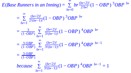
The resulting expectation creates a baseline for our pitcher’s performance by inning and allows us to determine if our starting pitcher generally meets or fails our expectations as the game progresses.

Table 3.1: Inning Base Runner Probabilities by Pitcher

	Tim Lincecum	Matt Cain	Jonathan Sanchez	Madison Bumgarner
P(O Base Runners)	0.333	0.352	0.280	0.356
P(1 Base Runner)	0.307	0.310	0.290	0.311
P(≥2 Base Runner)	0.360	0.338	0.430	0.333
E(Base Runners)	1.326	1.250	1.586	1.233

Based upon career OBPs through the 2013 season, Bumgarner would have the greatest chance (0.356) of retiring the side in order and he would be expected to allow the fewest base runners, 1.233, in an inning; Cain should also have comparable results. The implications are that Bumgarner and Cain represent a top tier of starting pitchers who are more likely to allow 0 base runners than either 1 base runner or +2 base runners in an inning. A pitcher like Lincecum, expected to allow 1.326 base runners in an inning, represents another tier who would be expected to pitch in the windup (for an entire inning) in approximately ⅓ of innings and pitch from the stretch in ⅔ of innings. Sanchez, on the other hand, represents a respectively lower tier of starting pitchers who are more likely to allow 1 or +2 base runners than 0 base runners in an inning. He has the least chance (0.280) of having a 1-2-3 inning and would be expected to allow more base runners, 1.586, in an inning.

As important as base runners are for turning into runs, the hits and walks that make up the majority of base runners are two disparate skills.  Hits generally result from pitches in the strike zone and demonstrate an ability to locate pitches, contrarily, walks result from pitches outside the strike zone and show a lack of command.  Hence, we’ll create an expectation for hits and another for walks for our starting pitchers to determine if they are generally good at preventing hits and walks or prone to allowing them in an inning.

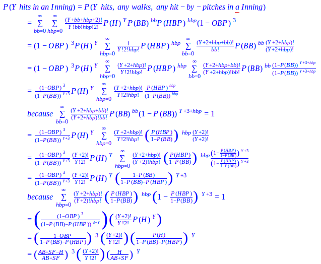
Let h, bb, and hbp be random variables for hits, walks, and hit-by-pitches and let P(H), P(BB), P(HBP) be their respective probabilities for a specific starting pitcher, such that OBP = P(H) + P(BB) + P(HBP). The probability of Y hits occurring in an inning for a specific pitcher can be constructed from the following negative multinomial distribution:

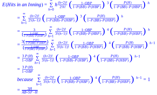
We can further apply the probability distribution above to create an expectation of hits per inning for our starting pitcher:

For walks, we do not have to repeat these machinations.  If we simply substitute hits for walks, the probability of Z walks occurring in an inning and the expectation for walks per inning for a specific pitcher become similar to the ones we deduced earlier for hits:

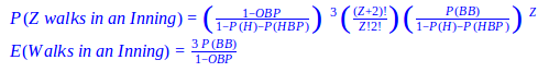
We could repeat the same substitution for hit-by-pitches, but the corresponding probability distribution and expectation are not significant.

Table 3.2: Inning Hit Probabilities by Pitcher

	Tim Lincecum	Matt Cain	Jonathan Sanchez	Madison Bumgarner
P(O Hits in 1 Inning)	0.457	0.466	0.439	0.443
P(1 Hits in 1 Inning)	0.315	0.314	0.316	0.316
P(2 Hits in 1 Inning)	0.145	0.141	0.152	0.150
P(3 Hits in 1 Inning)	0.056	0.053	0.061	0.060
E(Hits in 1 Inning)	0.896	0.870	0.947	0.936

The results of Table 3.2 and Table 3.3 are generated through our formulas using career player statistics through 2013. Cain has the highest probability (0.466) of not allowing a hit in an inning while Sanchez has the lowest probability (0.439) among our starters. However, the actual variation between our pitchers is fairly minimal for each of these hit probabilities. This lack of variation is further reaffirmed by the comparable expectations of hits per inning; each pitcher would be expected to allow approximately 0.9 hits per inning. Yet, we shouldn’t expect the overall population of MLB pitchers to allow hits this consistently; our the results only indicate that this particular Giants rotation had a similar consistency in preventing the ball from being hit squarely.

Table 3.3: Inning Walk Probabilities by Pitcher

	Tim Lincecum	Matt Cain	Jonathan Sanchez	Madison Bumgarner
P(O Walks in 1 Inning)	0.685	0.718	0.589	0.776
P(1 Walk in 1 Inning)	0.244	0.225	0.286	0.189
P(2 Walks in 1 Inning)	0.058	0.047	0.093	0.031
P(3 Walks in 1 Inning)	0.011	0.008	0.025	0.004
E(Walks in 1 Inning)	0.404	0.351	0.580	0.264

The disparity between our starting pitchers becomes noticeable when we look at the variation among their walk probabilities. Bumgarner has the highest probability (0.776) of getting through an inning without walking a batter and he has the lowest expected walks (0.264) in an inning. Sanchez contrarily has the lowest probability (0.589) of having a 0 walk inning and has more than double the walk expectation (0.580) of Bumgarner. Hence, this Giants rotation had differing abilities targeting balls outside the strike zone or getting hitters to swing at balls outside the strike zone.

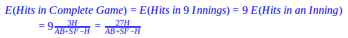
Now that we understand how a pitcher’s performance can vary from inning to inning, we can piece these innings together to form a 9 inning complete game. The 9 innings provides complete depiction of our starting pitcher’s performance because they afford him an inning or two to underperform and the batters he faces each inning vary as he goes through the lineup. At the end of a game our eyes still to gravitate to the hits in the box score when evaluating a starting pitcher’s performance.

Let D, E, and F be the respective hits, walks, and hit-by-pitches we expect to occur in a game, then the following negative multinomial distribution represents the probability of this specific 9 inning game occurring:

Utilizing the formula above we previously answered, “What is the probability of a no-hitter?”, but we can also use it to answer a more generalized question, “What is the probability of a complete game Y hitter?”, where Y is a random variable for hits. This new formula will not only tell us the probability of a no-hitter (inclusive of a perfect game), but it will also reveal the probability of a one-hitter, three-hitter, etc. Furthermore, we can calculate the probability of allowing Y hits or less or determine the expected hits in a complete game.

Let h, bb, hbp again be random variables for hits, walks, and hit-by-pitches.

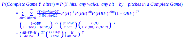
The derivations of the complete game formulas above are very similar to their inning counterparts we deduced earlier. We only changed the number of outs from 3 (an inning) to 27 (a complete game), so we did not need to reiterate the entire proofs from earlier; these formulas could also be constructed for an 8 inning (24 outs), a 10 2/3 inning (32 outs), or any other performance with the same logic.

Table 3.4: Complete Game Hit Probabilities by Pitcher using BA

	Tim Lincecum	Matt Cain	Jonathan Sanchez	Madison Bumgarner
P(O Hits in 9 Innings)	0.001	0.001	0.001	0.001
P(≤1 Hit in 9 Innings)	0.006	0.007	0.004	0.005
P(≤2 Hits in 9 Innings)	0.023	0.026	0.017	0.018
P(≤3 Hits in 9 Innings)	0.060	0.067	0.046	0.049
P(≤4 Hits in 9 Innings)	0.124	0.137	0.099	0.105
E(Hits in 9 Innings)	8.062	7.833	8.526	8.420

The results of Table 3.4 were generated from the complete game approximation probabilities that use batting average (against) as an input. Any of the four pitchers from the Giants rotation would be expected to allow 8 or 9 hits in a complete game (or potentially 40 total batters such that 40 = 27 outs + 9 hits + 4 walks), but in reality, if any of them are going to be given a chance to throw a complete game they’ll need to pitch better than that and average less than 3 pitches per batter for their manager to consider the possibility. If we instead establish a limit of 3 hits or less to be eligible for a complete game, regardless of pitch total, walks, or game situation (not realistic), we could witness a complete game in at most 1 or 2 starts per season for a healthy and consistent starting pitcher (approximately 30 starts with a 5% probability). Of course, we would leave open the possibility for our starting pitcher to exceed our expectations by throwing a two-hitter, one-hitter, or even a no-hitter despite the likelihood. There is still a chance! Managers definitely need to know what to expect from their pitchers and should keep these expectations grounded, but it is not impossible for a rare optimal outcome to come within reach.