Having grown up playing catcher from Little League through college, I always recognized the temptation and situational changes that occurred in terms of strategy and pitch selection with runners on, particularly base stealers, versus with no runners on base.  As a catcher, my thought process with a base stealer on, is always to try and have my pitcher get the ball to me as quickly as possible.  An earlier study I read dealt with the correlation between pitchers’ times to home, and that being a much stronger factor in throwing out a base-stealer than catcher pop times.  Logically, in thinking of pitch selection as a way of controlling the run game, the quickest way to get the catcher the ball is with one’s fastest pitch.

To evaluate the impact of base-stealers I defined a base stealer as a player who swiped 20 plus bags in 2013.  Using Baseball Reference, I slotted 6 pairs of base stealers and their following hitters.  The criteria for those hitters being 400 plus plate appearances in the same slot in the batting order.  Nick Swisher however is an exception because he had 250 plus appearances behind both Michael Bourn and Jason Kipnis, but I decided to include him.  I should also note that all the statistics in this study are from 2013.  Using Baseball Savant’s Pitch f/x database I defined a fastball as a 4 seam, 2 seam, sinker, splitfinger, and cutter and every other pitch as a breaking ball.  I then compared the fastball and breaking ball rates with each hitter with a runner on 1^st or nobody on.

It is taken from granted that for a hitter the best pitch to hit is a fastball.  While there are many different approaches, one of the most common is “fastball adjust,” meaning the hitter always looks, or anticipates, a fastball as you get in the box.  However, if you recognize something different out of the pitcher’s hand, you should have more time to adjust.  Hitters are always fastball hunters first, that’s why we call 2-0, 3-1 counts “hitter’s counts” because they will most likely get a fastball and at the same time are sitting fastball.  As proof we used the probability of scoring a run per 100 pitches of a certain pitch above the prototypical average players.  The league average probability of scoring runs against what I defined as a fastball type pitch for every 100 pitches in 2013 was 0.0167 and for every 100 off speed pitches was -0.07.  That is over an 8/100ths difference in the likelihood of scoring a run above average, which added up over the thousands of pitches a player can see a year can make an impact.  Below are the 6 hitters I used for this study and their run probability rates against different pitches:

As the data above supports, the best pitch to hit, the pitch a hitter is most likely to score more runs from, is a fastball.

So that being said, if a reputed, or habitual, base stealer is on base, then will the hitter at bat see an unusually high rate of fastball-like pitches?  With a higher rate of fastballs the hitter should therefore have a greater chance of success.  The theory being that an offense built more on speed and base stealing should see a higher rate of fastballs which then gives that team a greater probability of scoring more runs.

Now the total overall fastball rate for the league as a whole for the 2013 season was 57.8%.  The total fastball rates I arrived at were derived from simply taking the situational fastball rate and dividing it by the total pitch percentage or fastball percentage plus breaking ball percentage: fastball% / (fastball% + breaking ball%).

Looking at the results, in particular the totals, there is no significant difference in percentages of fastballs vs off speed seen with a runner on first or not.  The biggest difference is a 4.46% difference with David Wright.  And David Wright scores 21.1 runs above average against fastball type pitches (wFB).  While maybe an extra 4.46% increase does not make a world of difference it still contributes to overall run production and as we know in baseball 1 run can decide a game and 1 game can decide a season.  However, it appears that my hypothesis is false and there is no significant difference in situational pitch selection with a base stealer on 1^st.

Now I will be the first to admit that there are definitely ways to improve upon the accuracy of my theory.  The biggest problem being that I could not find a database on the internet that allowed me the option of isolating at bats with only specific runners on, so the next best thing was Baseball Savant’s option of isolating at bats with the option of runners on certain bases or a combination thereof.  So all these plate appearances measured are just with a generalized runner on 1^st who could be anybody or nobody on at all.  This study is assuming that the runner on 1^st, for a majority of the time, is the base stealer who hits 1 spot in front of the selected hitter.  BIG assumptions I realize.  Also this is only covering 6 hitters in their 2013 season, which is a small sample size considering.  Unfortunately I did not have all the resources necessary for the most accurate representation for this study as a whole and on that note I hope many of you who perhaps have more available to you, can dig deeper and build on my theory.

This is my first time posting something like this so if you have any helpful questions/comments/criticism/advice please feel free to comment.  And if you have a way to more thoroughly complete this study please do so!  Thanks and I hope you enjoyed.

Will Middlebrooks is a popular pick for a breakout player (at least according to the local Boston media).  Now breakouts aren’t really something you can predict, but I will not go into that whole can of worms.  On the surface Will Middlebrooks seems like an obvious choice, a young player with power, coming off a down year with no serious injury history.  The hopes for a Middlebrooks breakout upon closer inspection seem to be driven by hope and optimism rather than actual facts.

Middlebrooks’s glaring flaw last season was his sub .300 OBP (.271), which was driven in large part by his low walk rate (5.3%) and high strikeout rate (26.2%).  Believing that Middlebrooks can improve those numbers is central to any hope that he will have a breakout season.  Alex Speier  showed that it’s not unprecedented for young power hitters with sub .300 OBPs to see a large improvement in the OBP area, but it’s also not guaranteed.  Of the players Speier looked at only 18% saw their OBP increase by 30 points or more (which is what it would take to get Will over .300), so why does the Boston media believe that Middlebrooks will experience this rare transformation?

The main driving narrative behind this optimism is that Middlebrooks was over aggressive and had terrible plate discipline last year, and this allowed pitchers to dominate him. But now that he has worked on his approach at the plate during spring training everything will come together.

This “Willpower” narrative goes all the way to the top

Red Sox manager John Farrell told reporters “I think last year we saw some at-bats where maybe he was pressing a little bit, maybe trying to make up for some previous at-bats where it would cause him to be a little overaggressive or expand the strike zone, That willingness to swing, pitchers didn’t have to challenge him all that much” when explaining Middlebrooks past struggles.  We are led to believe that this former Achilles heel is no more after his successful spring training, as Middlebrooks told reporters “The one thing that sticks out to me is I’ve swung at one pitch outside of the zone this spring.”

Will Middlebrooks had a great spring training ( .353/.389/.667) but spring training stats are useless for predicting regular season success.  And, as it turns out, are far from the only problems with this “Willpower” narrative.  The idea that Will Middlebrooks was overly aggressive and had bad plate discipline is something that can be checked very easily by looking at Middlebrooks’s plate discipline stats vs the league average for last season.

Did Middlebrooks have poor plate discipline last season?

Will Middlebrooks plate discipline compared to the average major leaguer.

Checking the number reveals the surprising fact that Will Middlebrooks’s plate discipline was not terrible but surprisingly average.  He appeared to be a little bit aggressive, swinging a bit more at the first pitch but those 0.9 percentage points translated three more plate appearances with Will swinging at the first pitch hardly enough to ruin his triple slash line.  The next surprising thing that the numbers reveal is that pitchers were actually throwing Middlebrooks more strikes than the average hitter (and more compared to what he saw the previous season), so while pitcher might not have had to challenge him, they didn’t shy away from throwing him pitches in the zone.  Middlebrooks actually saw a lot more pitches in the strike zone than other power hitters.  For players with at least a 0.190 ISO and at least 350 PA only Jayson Werth saw more pitches in the strike zone .  These facts throw the whole premise of this “Willpower” out the window.

How does the image of Will Middlebrooks the aggressive hacker persist when it’s clearly untrue?

Well whenever you see such a low walk rate coupled with such a high strike out rate the easy first assumption is that the player swings at everything, this is a fare guess if didn’t have better data, but we do.  But what about some on who watched every single Middlebrooks plate appearance such as his manager, how could they have such a distorted view.  Well everything is relative, relative to an average major-leaguer Middlebrooks’s plate discipline and his approach were average but compared to other players on the Red Sox Middlebrooks was aggressive and undisciplined.  The Red Sox as a team swung at the first pitch less often than any other team in the majors.  So when not watching Middlebrooks, John Farrell was watching some of the most patient and disciplined hitters in baseball so this is an understandable bias.

The highly improbable feat of chasing only one pitch out of the strike zone over 26 plate appearances.

Now let’s look at Will’s assertion that he only chased one pitch out of the strike zone over his first 26 plate appearances (that’s the number he had prior to his quote).  This would be incredible and might even be meaningful if it were true.  We don’t have spring training plate discipline numbers so we will do a Gedankenexperiment (what Einstein called thought experiments because he was German) and assume the Will saw 100 pitches over those 26 plate appearances (lower than his career average rate and a bit below league average) and half of those were out of the strike zone (also generous considering that usually more than half of pitches are out of the strike zone and in spring pitcher are rusty and of a lower talent pool) this would give Will Middlebrooks a 2% chase rate ( chances are it would have to be lower than that for him to only chase one pitch over 26 plate appearances but we are giving him the benefit of the doubt).  This would be really impressive for a guy who normally chased around 30% of pitches (it would actually be impressive for anyone), and it’s a number that no one has ever sustained for a full season.

How rare is 2% chase rate over that short a time frame?  It’s so rare that no one even came close to it last year.  The closest was Shane Robinson, when last year in the month of June he had 27 plate appearances and only swung at 7.7% of pitches outside the strike zone, that was the lowest chase rate any player had during any month last season (assuming they had at least 20 plate appearances).

Given our prior knowledge about Will Middlebrooks and major-league hitters in general I will go out on a limb and say that I believe Middlebrooks swung at more than one pitch out of the zone.  I bet Middlebrooks believes he only swung at one pitch out of the zone, and this more than anything might point to a flawed understanding of the strike zone.  So while any player can improve by improving their plate discipline (case in point that Joey Votto can still benefit from it) its not a cure-all for baseball problems, and Will Middlebrooks’s problems extend beyond his plate discipline.

If plate discipline wasn’t the reason Middlebrooks was terrible last year then what was the problem?

Part of Middlebrooks’s problem was his abysmal .263 BABIP, this will likely be closer to league average in 2014 and is probably one of the best reasons to believe that Middlebrooks will be better than he was last year.  Unfortunately it sounds much better to say you are working on your plate discipline in spring training than to say you are hope your BABIP will regress towards the mean.  But BABIP is only part of the picture it doesn’t explain his 5.3% walk rate and 26.2% strikeout rate (the low BABIP and therefore production might have led pitcher to throw Will more strikes thus diminishing his walk rate, but this would only be a small effect).

Middlebrooks’s real problem seems to be with making contact, especially when it comes to pitches in the strike zone. He was 212th out of the 237 players with at least 350 PA last year in terms of zone contact (that means 89% of players are better than him), making contact only 81.4% of the time when he swung at a pitch in the strike zone.  This low zone contact rate is probably a large part of the reason pitchers felt comfortable throwing him so many pitches in the zone.  This issue was further compounded by the fact that when Will did make contact the ball went foul slightly more than half of the time (50.4% compared to the league average of 48.1%).  This leads to his high strike out rate.

Look at it this way:

a)      when Middlebrooks swung his chance of making contact with the ball was below average, and

b)      when he did make contact the chance of that ball going in fair territory was below average, and

c)       if that ball was put in play the chance of it being a hit was well below average.

These issues meant pitchers could throw Will lots of strikes, and if a player with average discipline sees fewer balls than average then they are going to walk less than average.

Will Middlebrooks will most likely be better than he was last season (more of a bounce-back than a breakout), and he might even have a breakout season but it will take more than improved plate discipline for that to happen.

All stats are from FanGraphs (used the regular plate discipline stats not the pitch f/x ones) with the exceptions of pitches per PA, 1^st pitch swing%, and foul ball stats which are all from baseball-reference.com

Also the quotes are from the Alex Speier article, although I believe they were given to the media in general.

Ever since Matt Holliday came into the league in 2004, he has been a model of consistency. His WAR increased after each of his first two seasons before peaking at 7.2 WAR in his fourth MLB season. Since reaching 7.2 WAR, Holliday has yet to fall below 4.5 WAR. While Holliday has yet to experience any significant declines in production, he has seen a few areas of his game begin to decline, especially in his power production. For a 34-year-old player, this is not incredibly surprising, but as a power hitter, it is a little concerning. With Holliday heading into his age-34 season, it is important to question whether he is still the model of consistency that he has been since reaching the MLB. For the 2014 campaign, the ZiPS Projection System sees Holliday declining a career high 1.4 wins all the way down to 3.1 WAR. This is still a very respectable total, but it is a quick drop for such a steady performer and could indicate further drops in production.

As I mentioned above, Holliday’s power production has been on a steady decline. His SLG% has declined for 3 straight seasons and settled in at .490 in 2013, which is his lowest SLG% since his rookie campaign in 2004. Holliday’s Isolated Power has dipped each of the past two seasons and even reached a career low of .190 in 2013. Both these numbers are very impressive, especially since they are at or near his career lows; however, they still represent an alarming trend with his power production. As would be expected with a lower SLG% and ISO, Holliday’s HR/FB% has declined for two straight seasons falling to 15%. While Holliday has never been considered a plus fielder, his UZR/150 has declined each of the last 3 seasons all the way down to -7.0. With all these statistics declining, Holliday’s WAR has dropped each of the past three seasons.

While Holliday has seen some dip in his power production, many other areas of his game have improved or stayed relatively constant. Also, despite his SLG and ISO declining, Holliday has still topped 20 homers in each of the past 8 seasons. He has also had a very healthy BB% since 2008, as it has remained above 10% each season and reached 11.5% in 2013, just under his career high of 11.9%. Even more impressive than his steady walk rate is that he lowered his K% to 14.3% in 2013, which was just above his career best K% of 13.8%. Altogether, Holliday was able to set a career best BB/K ratio of .80 in 2013.

In recent years Holliday has maintained both a high Batting Average and a high On-Base Percentage. Holliday has remained such a strong contributor at the plate, despite his worsening power, in large part because his OBP has remained extremely high. OBP is something that usually ages very well, which is encouraging for Holliday because so much of his offensive value hinges on his ability to reach base. In each of the last 7 seasons, Holliday’s wRC+ has been over 140 and was even 148 in 2013. For reference, 100 wRC+ is considered average, so 140 is excellent. There is no doubt that Holliday has remained an outstanding hitter over the past few years, but the real question is whether he will see a significant drop in production as he enters his age-34 season.

While his overall production has remained impressive, it is important to look at his contact rates and balls in play data in order to determine if this production is likely to continue. Throughout his career, Holliday has had an incredibly high Batting Average on Balls In Play (BABIP), with his career BABIP at .343. However, his BABIP dropped to a career low of .322 in 2013. Despite his BABIP falling from the previous season, he was still able to increase his batting average, which suggests he can continue to hit for a strong average even if his BABIP falls a little more. While his SLG and BABIP were down last year, Holliday actually increased his LD% above his career average, but also saw his Infield Flyball% (IFFB%) spike to 13.6%. Another encouraging sign with his LD% increasing was the fact that he also increased his Contact% to 81%, which marked a career high. His high contact rate no doubt helped him cut his K%, which will be important moving forward.

As Holliday continues to age into his mid-30’s, it will be interesting if he can remain the model of consistency that he has been for his entire career. It is clear that Holliday cannot sustain his current level of success for the remainder of his career, but little evidence suggests that 2014 will be the first year he experiences a significant drop in production. His lessening power is not a major concern to his overall game as long as he is able to maintain his high OBP skills and low K%. Turning back to the ZiPS projection of a 3.1 WAR, I do not see Holliday’s production taking that big of a hit, as their projection also calls for a .029 drop in OBP, which seems unlikely given his consistency in being able to get on base and the fact that OBP tends to age well. I expect Holliday to continue his slow decline, but I still see him posting a WAR above 4.0 and an OBP north of .375, especially if he can maintain a BB% in the double digits.

I. Introduction

A starting pitcher should have the advantage over opposing batters throughout a baseball game, yet as he pitches further into the game this advantage should slowly decrease.  The opposing manager hopes that his batters can pounce on the wilting starting pitcher before his manager removes him from the game.  But what would we see if the manager decided against removing his starting pitcher?  The goal of this analysis is to determine the consequences of allowing an average starting pitcher to pitch further into the game instead of removing him.  There are several different ways this situation can unfold for a starting pitcher, but we should be able to tether our expectations to that of an average starting pitcher.

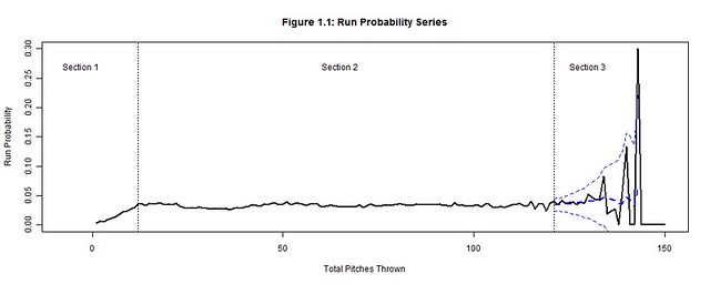
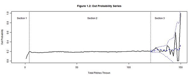
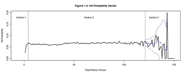
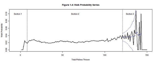
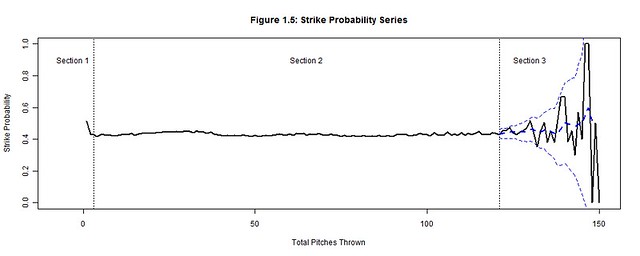
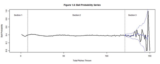
We will focus on how the total pitches thrown by starting pitchers (per game) affects runs, outs, hits, walks, strikes, and balls by analyzing their corresponding probability distributions (Figures 1.1-1.6) per pitch count; the x-axis represents the pitch count and the y-axis is the probability of the chosen outcome on the i^th pitch thrown.  Each plot has three distinct sections:  Section 3 is where the uncertainty from the decreasing pitcher sample sizes exceeds our desired margin of error (so we bound it with a confidence interval); Section 1 contains the distinct adjustment trend for each outcome that precedes the point where the pitcher has settled into his performance; Section 2, stable relative to the others sections, is where we hope to find a generalized performance trend with respect to the pitch count for each outcome.  Together these sections form a baseline for what to expect from an average starting pitcher.  Managers can then hypothesize if their own starting pitcher would fare better or worse than the average starting pitcher and make the appropriate decisions.

II.  Data

From 2000-2004, 12,138 MLB games were played; there should have been 12,150 games but 12 games were postponed and never made up.  During this period, starting pitchers averaged 95.12 pitches per game with a standard deviation of 18.21.  The distribution of pitch counts is normal with a left tail that extends below 50 pitches (Figure 2).  It is not symmetric about the mean because a pitcher is more likely to be inefficient or injured early (left tail) than to exceed 150 pitches.  In fact, no pitcher risked matching Ron Villone’s 150 pitch count from the 2000 season.

This brief period was important for baseball because it preceded a significant increase in pitch count awareness.  From 2000-2004, there averaged 192 pitching performances ≥122 pitches per season (Table 2); 122 is the sampling threshold explained in the next section.  Since then, the 2005-2009 seasons have averaged only 60 performances ≥122 pitches per season.  This significant drop reveals how vital pitch counts have become to protecting the pitcher and controlling the outcome of the game.  Now managers more frequently monitor their pitchers’ and the opposing pitchers’ pitch counts to determine when they will expire.

Table 2:  2000-2009 Starting Pitcher Pitch Counts ≥122

III. Sampling Threshold (Section 3)

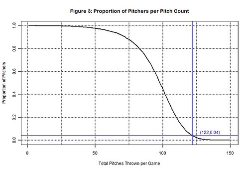
122 pitches is the sampling threshold deduced from the 2000-2004 seasons (and the pitch count minimum established for Section 3), but it is not necessarily a pitch count threshold of when to pull the starting pitcher.  Instead this is the point when starting pitcher data becomes unreliable due to sample size limitations.  Beyond 122 pitches, the probabilities of Figures 1.1-1.6 violently waver high and low as very few pitchers threw more than 122 pitches.  A smoothed trend, represented by a dashed blue line and bounded by a 95% confidence interval was added to Section 3 of Figures 1.1-1.6 to contain the general trend between these rapid fluctuations.  But the margin of error (the gap between the confidence interval and the smoothed trend) grows exponentially beyond 3%, so the actual trend could be anywhere within this margin.  Thereby, we cannot hypothesize whether it is more or less likely that the pitcher’s performance will excel or plummet after 122 pitches.

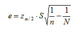
To understand how the 122 sampling threshold was determined, we first extract the margin of error formula (e) from the confidence interval formula (where  z_α/2 = z-value associated with the (1-α/2)^th percentile of the standard normal distribution, S = standard error of the sample population, n = sample size, N = population size):

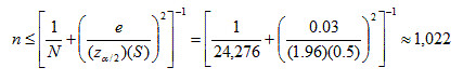
Next, we back-solve this formula to find the maximum sample size n for when the margin of error exceeds 3%; we use S = 0.5, z_2.5% = 1.96, N = 2 pitchers × 12,138 games = 24,276:

There is no pitch count directly associated with the sample size of 1,022, but 1,022 can be bounded between the 121 (n=1,147) and 122 (n=971) pitch counts.  At 121 pitches the margin of error is still less than 3%, but it becomes greater than 3% at 122 pitches and begins to increase exponentially.  This is the point the sample size becomes unreliable and the outcomes are no longer representative of the population.  Indeed only 4% (971 of 24,276) of the pitching performances from 2000-2004 equaled or exceeded 122 pitches thrown in a game (Figure 3).

A benefit of the sampling threshold is that it separates the outcomes we can make definitive conclusions about (<122 pitches) from those we cannot (≥122 pitches).  If were able to increase the sampling threshold another 10 pitches, we could make conclusions about the throwing up to 131 pitches in a game.  However, managers will neither risk the game outcome nor injury to their pitcher to accurately model their pitcher’s performance at high pitch counts.  Instead, the sampling thresholds have steadily decreased since 2005 and the 2000-2004 period is likely the last time we’ll be able to make generalizations about throwing 121 pitches in a game.

Yet, even for the confident manager, 121 pitches is still a fair point in the game to assess a starting pitcher.  Indeed the starting pitcher must have been consistent and trustworthy to pitch this deep into the game.  But if the manager wants to allow his starting pitcher to continue pitching, he is only guessing that this consistency will follow because there is not enough data to accurately forecast his performance.  Instead he should consider replacing his starting pitcher with a relief pitcher.  The relief pitcher is a fresh arm that offers less risk; he must have a successful record based on an even smaller sample size of appearances, smaller pitch counts, and a smaller margin of error.  The reliever and his short leash are the surer bet than a starting pitcher at 122 pitches.

IV.  Adjustment Period (Section 1)

The purpose of the adjustment period is to allow the starting pitcher a generous period to find a pitching rhythm.  No conclusions are made regarding the probabilities in the adjustment period as long as an inordinate amount of walks, hits, and runs are not allowed.  The most important information we can impart from this period is the point when the adjustment ends.  Once the rhythm is found, we can be critical of a pitcher’s performance and commence the performance trend analysis.

In order to be effective from the start, starting pitchers must quickly settle into an umpire’s strike zone and throw strikes consistently; most pitchers do so by the 3^rd pitch of the game (Figure 1.5).  Consistent strike throwing keeps the pitcher ahead in the count and allows him to utilize the outside of the strike zone rather than continually challenging the batter in the zone.  Conversely, a pitcher must also include (pitches called) balls into his rhythm, starting approximately by the 8^th pitch of the game (Figure 1.6).  Minimal ball usage clouds the difference between strikes and balls for the batter while frequent usage hints at a lack of control by the pitcher.  Strikes and balls furthermore have a predictive effect on the outcomes of outs, hits, runs, and walks:  a favorable count for the batter forces the pitcher to deliver pitches that catch a generous amount of the strike zone while one in favor of the pitcher forces the batter to protectively swing at any pitch in proximity of the strike zone.

On any pitch, regardless of the count, the batter could still hit the ball into play and earn an out or hit.  Yet as long as the pitcher establishes a rhythm for minimizing solid contact by the 4^th pitch of the game (Figure 1.2-1.3), he can decrease the degree of randomness that factors into inducing outs and minimizing hits.  A walk contrarily cannot occur on any pitch because walks are the result of four accumulated balls.  Pitchers should settle into a rhythm of minimizing walks by using minimal ball usage; so when the ball rhythm stabilizes (on the 8^th pitch of the game) the walk rhythm also stabilizes (Figure 1.4).  After each of these rhythms stabilizes, a rhythm can be established for minimizing runs (a string of hits, walks and sacrifices within an inning) by the 12^th pitch of the game (Figure 1.1).  It is possible for home runs or other quick runs to occur earlier, but pitchers who regularly put their team in an early deficit are neither afforded the longevity to pitch more innings nor the confidence to make another start.

V.  Performance Trend (Section 2)

Each of the probability distributions in Figures 1.1-1.6 provides a generalized portrayal of how starting pitchers performed from 2000-2004, but in terms of applicability they do not depict how an average starting pitcher would have performed.  Not all pitchers lasted to the same final pitch (Figure 2).  The better a pitcher performed the longer he should have pitched into the game, so we would expect each successive subset of pitchers (lasting to greater pitch counts) to have been more successful than their preceding supersets.  Thereby, in order to accurately project the performance of an average starting pitcher the probability distributions need to be normalized, by factors along the pitch count, as if no pitchers were removed and the entire population of pitchers remained at each pitch count.

The pitch count adjustment factor (generalized for all pitchers) is a statistic that must be measurable per pitch rather than tracked per at-bat or inning, so we cannot use batting average, on-base percentage, or earned run average.  The statistic should also be distinct for each outcome because a starting pitcher’s ability to efficiently minimize balls, hits, walks, and runs and productively accumulate strikes and outs are skills that vary per pitcher.  Those who are successful in displaying these abilities will be allowed to extend their pitch count and those who are not put themselves in line to be pulled from the game.

We accommodate these basic requirements by initially calculating the average pitches per outcome x, R_x(t), for any pitcher who threw at least t pitches (where PC_t = sum of all pitch counts and x_t = sum of all x for all pitchers whose final pitch was t):

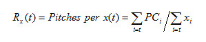
This statistic, composed of a starting pitcher’s final pitch count divided by his cumulative runs allowed (or the other outcome types), distinguishes the pitcher who threw 100 pitches and allowed 2 runs (50 pitches per run) versus the pitcher with 20 pitches and 2 runs (10 pitches per run).  At each pitch count t, we calculate the average for all starting pitchers who threw at least t pitches; we combine their various final pitch counts (all ≥t), their run totals (occurring anytime during their performance), and take a ratio of the two for our average.  At pitch count 1, the average is calculated for all 24,276 starting pitcher performances because they all threw at least one pitch; the population of starting pitchers allowed a run every 32.65 pitches (Table 5.1).  At pitch count 122, the average is calculated for the 971 starting pitcher performances that reached at least 122 pitches; this subset of starting pitchers allowed a run every 57.75 pitches per game.

Table 5.1:  2000-2004 Pitches per Outcome

Starting pitchers will try to maximize the pitches per outcome averages for runs, hits, walks, and balls while minimizing the probabilities of these outcomes, because the pitches per outcome averages and the outcome probabilities have an inverse relationship.  Conversely, starting pitchers will also try to minimize the pitches per outs and strikes while trying to maximize these probabilities for the same reason.  Hence, we must invert the pitches per outcome averages into outcomes per pitch rates, Q_x(t), to be able to create our pitch count adjustment factor, PCA_x(t), that will compare the change between the population of starting pitchers and the subset of starting pitchers remaining at pitch count t:

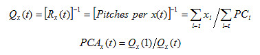
The ratio of change is calculated for each outcome x at each pitch count t.  The pitch count adjustment factor, PCA_x(t), will scale p_x(t), the original probability of x from the starting pitchers at pitch count t back to the expected probability of x for an average starting pitcher from the entire population of starting pitchers at pitch count t.

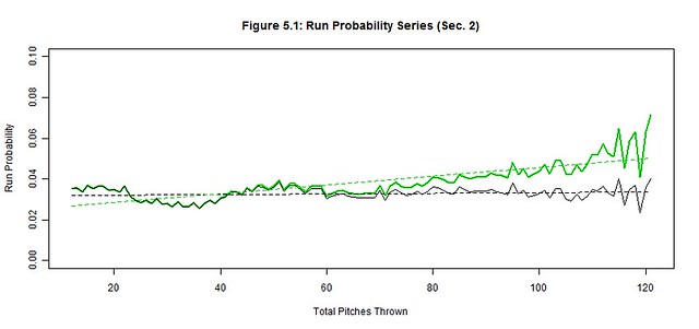
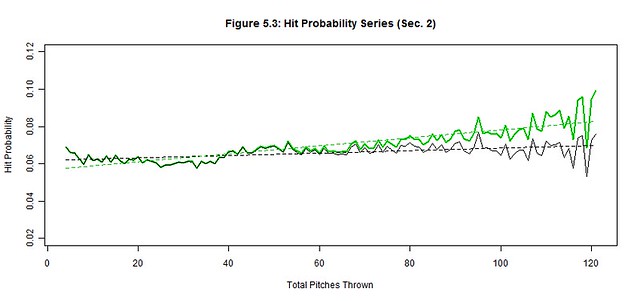
The increases to the pitches per run and pitches per hit rates strongly suggest that the 971 starting pitchers remaining at 122 pitches were more efficient at minimizing runs and hits than the overall population of starting pitchers.  The population performed worse than those pitchers remaining at 122 pitches by factors of 176.85% and 131.98% with respect to the runs per pitch and hits per pitch rates (Table 5.2).  Thereby, we would expect the probability of a run to increase from 3.40% to 6.01% and the probability of a hit to increase from 7.21% to 9.51% if we allowed an average starting pitcher from the population of starting pitchers to throw 122 pitches.

Table 5.2:  2000-2004 Average Pitcher Probabilities at 122 Pitches

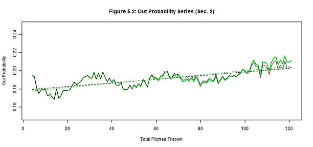
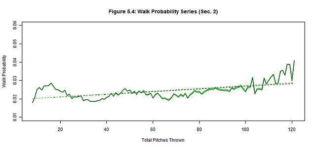
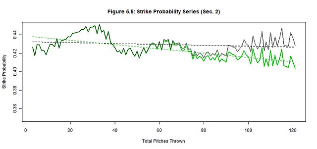
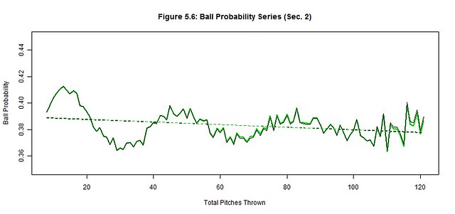
We apply the pitch count adjustment factors, PCA_x(t), at each pitch count t to each of the original outcome probability distributions (black) to project the average starting pitcher outcome probabilities (green) for Section 2 (Figures 5.1-5.6); the best linear fit trends (dashed black and green lines) are also depicted.  The reintroduction of the removed starting pitchers noticeably worsened the hit, run, and strike probabilities and slightly improved the out probability in the latter pitch counts.  There were no significant changes to ball and walk probabilities.  These are the general effects of not weeding out the less talented pitchers from the latter pitch counts as their performances begin to decline.

Next we quantify our observations by estimating the linear trends of each original and average pitcher series and then compare their slopes (Table 5.3).  The linear trend (where t is still the pitch count) provides a simple approximation of the general trend of Section 2 while the slope of the linear trend estimates the deterioration rate of the pitcher’s ability to control these outcomes.  The original pitcher trends show that the way managers managed pitch counts, their starting pitchers produced relatively stable probability trends as if the pitch count little or no effect on their pitchers; only the out trend changed by more than 1% over 100 pitches (2.00%).  Contrarily, the average pitcher trends increased by more than 2% over 100 pitches for the run, out, hit, and strike trends, indicating a possible correlation between the pitch count and the average pitcher performance; the walk and ball trends were unchanged from the original to the average starting pitcher.

We must also measure these subtle changes between the original and average trends that occur in the latter pitch counts of Figures 5.1-5.6.  There is rapid deterioration in the ability to throw strikes and minimize hits and runs between the original and average starting pitchers as suggested by the changes in slope.  The 368.21% change in the strike slopes clearly indicates that fewer strikes are thrown by the average starting pitcher in the latter pitch counts.  The factors of 222.53% and 1206.13% for the respective hit and run slopes indicate that the average starting pitcher is not only giving up more hits but giving up more big hits (doubles, triples, home runs).  There is a slight improvement in procuring an out (14.45%), but the pitches that were previously strikes became hits more often than outs for the average starting pitcher.  Lastly, the abilities to minimize balls (4.87%) and walks (8.23%) barely changed between pitchers, so control is not generally lost in the latter pitch counts by the average starting pitcher.  Therefore, the average starting pitcher isn’t necessarily pitching worse as the game progresses but the batters may be getting better reads on his pitches.

Table 5.3:  Section 2 Linear Trend

The correlation coefficients also support our assertion that the average starting pitcher became adversely affected by the higher pitch counts, but even the original starting pitcher showed varied signs being affected by the pitch counts.  There were moderate correlations between the pitch count and hit and walks and a very strong correlation between the pitch count and outs.  So even though some batters improved their ability to read an original starting pitcher’s pitches, this improvement was not consistent and the increases to hits and walks were only modest.  Contrarily, the original starting pitcher did become more efficient and consistent at procuring outs as the pitch count increased.   We also found weak correlations between the pitch count and strikes and balls for the original starting pitcher, so strikes and balls were consistently thrown without any noticeable signs of being affected by the pitch count.   However, out of all of our outcomes, the pitch count of the original starting pitcher had the weakest correlation with runs.  Either the original starting pitchers could consistently pitch independent of the pitch count or their managers removed them before the pitch count could factor into their performance; the latter most likely had the greater influence.

It is also worth noting the intertwined patterns displayed in Figures 5.1-5.6 and Table 5.1.  Strikes and balls naturally complement each other, so it should come as no surprise that the Strike Probability Series and Ball Probability Series also complement each other; a peak in once series is a valley in the other and vice-versa.  The simple reason is that strikes and balls are the most frequent and largest of our outcome probabilities – they are used to setup other outcomes and avoid terminating at-bats in one pitch.  However, fewer strikes and balls are thrown in the latter pitch counts as evidenced by the decline in the Strike and Ball Probability Series, which make the at-bats shorter.  Consequently, there are fewer pitches thrown between the outs, hits, and runs, so these other probability series increase.  Hence, the probabilities of outs, hits, and runs become more frequent per pitch as the pitch count increases (further supported by the drop in pitches per strike and ball rates in Table 5.1).

VI.  Conclusions

Context is very important to the applicability of these results, without it we might conjecture that these trends would continue year over year.  Yet, the 2000-2004 seasons were likely the last time we’ll see a subset of pitchers this large pitching into extremely high pitch counts.   Teams are now very cautious about permitting starting pitchers to throw inconsequential innings or complete games, so the recent populations of starting pitchers have shifted away from the higher pitch counts and throw fewer pitches than before.  Yet, these pitch count restrictions should not affect the stability of our original probability trends.  The sampling threshold will indeed lower and the length of stable Section 2 will shorten, but the stability of the current original trends should not compromise.  Capping the night sooner for the starting pitchers only means they are less likely to tire or be read by batters.

We also cannot generalize that these original probability trends would be stable for any starting pitcher.  The probability trends and their stability are only representative of the shrinking subset of starting pitchers before their managers removed them due to performance issues, injury, strategy, etc.  These starting pitchers subsets may appear unaffected by the pitch count, but their managers created this illusion with the well-timed removal of their starting pitchers.  They understand the symptoms indicative of a declining pitcher and only extend the pitch count leash to starting pitchers who have shown current patterns of success.  Removing managers from the equation would result in an increased number of starting pitchers faltering in the latter pitch counts as their pitches are better read by batters.  Likewise, any runners left on base by the starting pitcher, but now the responsibility of a relief pitcher, would have an increased likelihood of scoring if the starting pitchers were not removed as originally planned by their managers.  Starting pitchers do notice these symptoms and may gravitate to finishing another inning, but each additional pitch could potentially damage the score significantly.  Trust in the manager and let him bear the responsibility at these critical points.

A couple years ago, The Oakland Athletics extended the contract for general manager Billy Beane for an additional 5 years, securing him through the 2019 season. They did not release the specific details of the contract, but we can guess that it’s comparable to the $3-4m that Brian Cashman and Theo Epstein make per year. The A’s are paying Alberto Callaspo $4.1m this year. Neither Beane’s nor Callaspo’s salary is particularly surprising, since both roughly reflect the current market for a top-tier GM and a 30-year-old infielder with a career .273/.335/.381 slash line. But is this reasonable? Should the owner of a baseball team be more willing to pay a mediocre infielder than an elite general manager? If the following data on front office success is any indication, absolutely not.

Using payroll data that goes back to 1998, I wanted to compare how well teams achieved success relative to the budgets they were given by their owner. In order to do so, I ran a regression model for every season to determine what sort of an effect payroll had on wins. For each season, the league average payroll is normalized to “1” to allow every season to be in this chart. As the graph shows, teams with more money tend to win more. If you’re adventurous and feel like interacting with the data you see below, click here and mouse over everything until you pass out.

It’s no surprise that money leads to success, and the fact that certain GMs tend to outperform their budget shouldn’t stun you either. But the extent to which some general managers are better than others is enormous. There are plenty of GMs who did exactly what you’d expect given their budgets. In 9 seasons with the Expos and Mets, Oscar Minaya was given the funds to win 742 games. He won 739. Mark Shapiro was supposed to win 703. He won 704.

Some general managers have better reputations, though. Theo Epstein, former Red Sox GM and current Cubs President of Baseball Operations, was given the budgets that would have resulted in 795 wins from an average GM, but he turned that into 839 wins in Boston. Legendary Braves GM John Schuerholz led a Braves squad that won 78 more games than expected since 1998, when the data begins. The 2nd best on the list, ex-Cardinals and current Reds GM, Walt Jocketty, has been worth an astounding 106 wins.

Then there’s Billy Beane: the Billy Beane who the A’s are paying slightly less than Alberto Callaspo. Under his direction, the Oakland Athletics have won 171 more games than expected. Babe Ruth had a career WAR of 168. Ruth’s best season was worth an absurd 15.0 wins in terms of WAR. Billy Beane has had 6 seasons during which the A’s won 15+ more games than they should have. They’ve never had the money to win 50% of their games, but half their seasons have ended with 20 more wins than losses.

I could go on. But first, let’s look at some visuals.

Here are the 16 general managers whose teams have exceeded their financial expectations by over 25 wins since 1998. If you want to look at every general manager’s wins and expected wins, explore this. One name I have not mentioned so far that has had an impressive stint as head of the Rays is Andrew Friedman. Since he’s been the GM of the Rays, they have been tied with St. Louis as the most cost effective winners in baseball. It’s even more impressive when you consider the dumpster fire he inherited.

After ignoring the potential for mediocrity during his first two seasons and building for the future, Friedman’s Rays took off. In the past 6 years, the Rays have won 87 more games than they should have. While it’s not as good as Beane’s best 6-year stretch of 117, it has coincided with a relatively weak stretch for the A’s where they have only exceeded their budget-wins by 30 games.

Unfortunately, not every team can have a Billy Beane or an Andrew Friedman. Some teams, like my Royals, have had more struggles. This chart, as much as anything else, shows the overwhelming need for effective front office management.

The A’s have been 300 wins more effective than the Orioles the last 16 years. If a win is worth $5m as recent free agency has suggested, then I don’t even want to type how much Billy Beane is worth. If you’re like me, it’s worth your time to explore this chart which shows yearly expectations and results for each team. A couple teams to look for, in addition to the ones I’ve talked about: the Cardinals and Braves have been unsurprisingly excellent, and the Cubs, Royals, and Orioles are worth looking at for less exciting reasons.

So how much should teams be paying their GMs? At this point, that’s an easy answer. $1 more than everyone else will pay, because they are tremendously undervalued right now. After that, the answer isn’t as clear, but I don’t see why they wouldn’t be similarly paid to players. One easy counter argument would be that if you pay the GM too much, he can’t do his job as well because he would have less money with which to pay players. But I think there is sufficient evidence that, for example, the Blue Jays would win more games with the team that Andrew Friedman could assemble with a $97m payroll than their current $117m team. The fact that the Rays will pay $57m this year for their squad should support that claim more than enough.

The free agent market would say that an elite GM could be worth $50-$100m a year. While that might strike people as unreasonable, it’s probably closer to their real value than the replacement level infielder-pay they are receiving now.

If you’re anything like most fantasy players, you may find yourself investing in similar players across multiple leagues. If you’re anything like me, those players seem to get injured more than others. If you are me, this year you invested in Mat Latos and Doug Fister everywhere you could… and are furious.

But if you need a placeholder for April while your starters heal, full-season projections might not be as relevant to your replacement decisions. While it’s always smart to go with skill as your primary determination, often the free agent pitching pool is fraught with pitchers that are more similar. In such instances, the pitcher’s April schedule could be of use. If you need a pitcher for one month and one month only, his May – September prospects are of little concern.

Either because I’m a simple man, or because I’m receiving $0 in compensation for this short piece, I decided a fair estimator would be to simply use the FanGraphs 2014 Projected Rankings and input each opponents Runs Scored per Game (RS/G) for each team on a schedule grid for the month of April. I then averaged out the projected RS/G of all opponents for each game in April. This is what I found.

What do we see here? First, as expected, on average the AL teams face more projected runs. You’re welcome for that valuable information. One interesting note, though, is that the San Francisco Giants will face an even tougher aggregate offense than four AL teams. What do we take from this? Maybe if you’re thinking about Tim Hudson vs. Marco Estrada in a shallow league for a rental, you take Hudson. In a shallower league in which this is a real decision, however, you can probably stream matchups with a high efficacy throughout the month. But as a FanGraphs reader (ego-stroke), there’s a fairly high probability that your most difficult decisions come in deeper leagues. So we shall redirect our attention to pitchers farther down the ranks.

“But DomRep,” you might smirk, “aren’t AL/NL differences factored into preseason rankings to a large degree?” Yes, observant reader, they are. This is why this table is much more useful when comparing pitchers in the same league. The NL is below:

In the NL, there may be a built-in feeling that, when two pitchers are similar, you’re probably better off just taking the guy from San Diego. Poppycock! San Diego will face the Dodgers, Brewers, and two AL teams this month (Tigers and Indians). Exclamation point! It should be noted that San Diego likely has a less pitcher-friendly park factor than they used to, but even still, a quick glance at the table above should help you decide to maybe choose Jhoulys Chacin, Taylor Jordan, or Tanner Roark over Eric Stults if you think they’re similar pitchers.

Here’s the AL:

In the A.L., one might take a quick gander and be encouraged to use Garrett Richards over Bud Norris because they face the easiest and toughest April pitching schedules, respectively. Pseudo-sleeper Tyler Skaggs might also be expected to start out well.

As we mentioned before, preseason rankings and projections take league into consideration. So when considering two pitchers in different leagues, it might even help to take a quick peek at their respective schedule rankings within their own league. For instance, while San Diego (#14 NL schedule) can be expected to face less run-scoring potential this month on average than Anaheim (#1 AL schedule), this will be the case the whole season and is, therefore, factored in when rankings show Tyson Ross and Tyler Skaggs in similar places. But the rankings eke out that Ross’s month should be harder than his average month while Skaggs’s month should be easier.

If you’re in a position to stream relatively strong pitchers throughout April, this is probably useless to you. The sample size of a month’s worth of starts can also blow all of this up. It’s common practice to look at September strength of schedule for pitchers, but everyone tends to ignore April because their eyes are focused on the whole season. But if you’re anything like me, and Latos/Fister are giving you fits, hopefully you’ll keep strength of schedule in mind.

I’m entering my fourth season of fantasy baseball this year and in my quest for my first championship I stepped up my preseason work to include making my own projections for players and creating my own dollar value system for my league’s custom scoring (6×6, standard with OPS and K/9 added). When making projections for players this year, I looked at their last three seasons in the Majors and used their Steamer and ZiPS projections to make sure I was in the same universe or had solid reasons for my different projection. I made projections for about 300 hitters and 200 pitchers, which I feel are grounded in reality and will give me an edge in my fantasy endeavors this year.

However, while I’m pleased with my projections and it’s definitely better than when I first started playing and just knew Yankees and other AL East players, my projections are still very limiting. One of the main problems is that I’m producing a single stat line for each player. It’s based on what they’ve done previously, how they’re trending, and how I and other systems think they’re mostly likely to produce in 2014, but it’s still just a single projection. More advanced projection systems, like PECOTA, compare a given player to thousands of other Major Leaguers to find comparable careers and produce various projections and each projections probability of occurring.

Projection systems like this recognize the inherent uncertainty of projecting future baseball performance and instead of giving one stat line, give us a range of outcomes with their likelihood and produce more accurate results. Now, I am just dipping my toe in the water of finding comparable players and making projections based on that but I wanted to see how this type of system would change my valuation two outfielders who will turn 27 this season, Justin Upton and Jay Bruce. Bruce will turn 27 in April and Upton turns 27 in August. They’ve both been big fantasy contributors in the past, Bruce is more consistent in his production while Upton has been streakier, with hot and cool months and peaks and valleys of home run and stolen base totals. I’ve put my projections for them below with a dollar value based on a 12 team league with 22 roster spots and a 70-30 hitters-pitchers split.

I’m projecting them to produce similar value, but Bruce definitely has an edge. To find comparable players to Bruce and Upton, I looked at all MLB season from 1961 through 2013 (61 being an arbitrary start date based on how much data my laptop could sort through and organize with John Henrying it’s CPU). I narrowed down to players with similar home run and stolen base totals in their age 23 to 26 seasons, along with average, OPS, strikeout and walk percentages, and playing time in an attempt to find a list of similar hitters.

For Jay Bruce I found 19 comps and I found 26 for Upton, there’s a link to the google doc with the full list below which I recommend checking out, it’s not included here so I can save some space. Now that I have the comparable players, I want to see how the performed in their age 27 season to give me a range of outcomes for both Bruce and Upton. I’ve included some bullet points here, again with the full spreadsheet linked at the end.

Mean and Median Value of Comparable Players’ Age 27 Season

• The average dollar value of Upton comparables was $27.17 and the median value was $31.49.
• The average of Bruce comparables was $21.39 and the median value was $19.51.

Best Case Scenario

• The best case scenario for Upton would be to follow Bobby Bonds’ age 27 season, where he put together his power and speed (39 HRs and 43 SBs) and bumped his average up to .283 from .260 in the previous year. I don’t think the HR total is out of the question, definitely hard and more than I’m predicting, and I think the average is within reach, but Bonds was regularly stealing 40 bases a year at this point which Upton is clearly not.
• The best case scenario for Bruce would be to follow Dale Murphy’s age 27 season. Murphy hit .302 that year, with 36 HRs, scoring 130 times and driving in 121 RBIs. While a .300 average may seem unfathomable for Bruce, Murphy hit .281 the year before and .247 the year before that. What makes this situation most unlikely, is that Murphy had a little more speed than Bruce (most seasons stealing bases totaling in the high single digits or low double digits) but he swiped 30 when he was 27, probably out of Bruce’s reach.

More Realistic Good Scenarios

• While I don’t expect Upton to reach Bobby Bonds level, it’s not hard to imagine him producing a line similar to Reggie Jackson’s 1973 when Jackson was 27. From 1970 to 1972, Jackson’s home run highs and lows by season were 23 to 32, his stolen bases ranged from 26 to 9, and his average fluctuated from .237 to .277.  There’s the volatile situation that we’ve grown accustomed to seeing from Upton. In 1973, Jackson put it together and hit 32 dingers, stole 22 bags, and hit .290.  Upton has already produced remarkably similar lines (2011 – 31HR/21SB/.289 avg) and could put it together for 2014.
• Jay Bruce isn’t going to steal 30 bases but he easily follow the 27 year old season of a former Cincinnati Red, Adam Dunn. Dunn was reliably hitting 40 home runs a year at this point (seriously, four straight season with exactly 40) and while Bruce has yet to reach the 40 mark, it’s not outside the realm of possibilities. The big difference with Dunn’s age 27 season from his other years is that he got his average up to .260 (bookended with .230 seasons), stole 9 bases, and had over 100 runs and RBIs. With Bruce entering his power prime, I think 40 homers is definitely possible, if still unlikely, and hitting .260 is definitely in his wheel house.

Outside of Injury, Worst Case Scenario

• For Upton, if he stays healthy the worst case scenario is following former Phillies 2B, Juan Samuel. Samuel had between .264 and .272 the four previous season, with home run totals as high as 28 but reliably in the high teens, and had stolen at least 30 bases each year. At age 27 though, his average fell to .240, he only hit 12 home runs (and never exceeded 13 again), and while he could rely on his speed and stole 30 bases he failed to produce 70 runs or RBIs. Not the most likely situation for Upton, but I could envision it with less stolen bases.
• For Bruce, the floor doesn’t get that low. If he reaches 500 Abs the worst comparable is Torii Hunter’s age 27 season where he only hit .250 and stole 6 bags, but still hit 26 homers and drove in 100 RBIs. Given Bruce’s consistency and the consistency of his comparables, I’d expect a high floor.

The Merciful Conclusion

 I know this took up a lot of room and we’re all happy this is almost over, but what does this mean. First, this is pretty rudimentary with no set formula for finding comparable players, I did my best but they’re definitely not one to one matches and should be taken with a grain of salt. However, I think this helps articulate a fundamental difference between Jay Bruce and Justin Upton. Bruce is a high floor, more limited ceiling guy and I’ve got more confidence that his 2014 will fall close to my projections. I know I’m buying about a .260 average, with a couple of stolen bases, mid 30s home runs with a little wiggle room, in a good lineup.

Justin Upton is a lotto ticket guy. I’m sticking with my projection for his season which falls between the extremes, but if he repeats his 2011 or puts together his tools that he has demonstrated at different points of his career, he could finish right behind Mike Trout among fantasy outfielders. At the same time, I could see him producing a line like his big brother BJ did last year, okay maybe not that bad, but definitely not worth his draft price. Who you take depends on what path you want to believe and who you already have on your team, but I think laying out these options and using player comparables definitely adds to fantasy projections and will be a staple I’ll use next year.

As promised, here’s the link to the full list of comparable players used for this article: https://docs.google.com/spreadsheet/ccc?key=0AmP-CH5MqzENdFZSZ0xhQVZiYWxNSVQxYzBsOFh3YkE#gid=0

Over the last decade, Fielding Independent Pitching (FIP) has become one of the main tools to evaluate pitchers. The theory behind FIP and similar Defensive Independent Pitching metrics is that ERA is subject to luck and fielder performance on balls in play and is therefore a poor tool to evaluate pitching performance. Since pitchers have little to no control over where batted balls are hit, we should instead look only to the batting outcomes that a pitcher can directly control and which no other fielder affects. In the case of FIP, those outcomes are home runs, strikeouts, walks, and hit batters.

However there are many serious issues with FIP that collectively make me question its usage and value. These issues include the theory behind the need for such a statistic, the actual parameters of the formula’s construction, and the mathematical derivation of the coefficients. Let’s address these issues individually.

Control over Balls in Play

A common statement when discussing FIP or BABIP is that pitchers have little to no control over the result of a ball once it is hit into play. A pitcher’s main skill is found in directly controllable outcomes where no fielder can affect the play, such as home runs, strikeouts, and walks (and HBP). In trying to estimate a pitcher’s baseline ERA, which is the objective of FIP, the approximately 70% of balls that are put into play can be ignored and we can focus only on the previously mentioned outcomes where no fielder touches the ball.

The concept of control is a little fuzzy though and something I believe has been misappropriated. It is definitely true that the pitcher does not have 100% absolute control over where a batted ball is hit. There is no pitch that anyone can throw that can guarantee a ball is hit exactly to a particular spot. However in the same vein, the batter doesn’t have 100% absolute control either. If you were to place a dot somewhere on the field, no batter is good enough to hit that spot every time, even if hitting off a tee.

However this lack of complete control should not in any way imply that the batter or pitcher doesn’t have any control at all over where the ball is hit. Batters hit the ball to places on the field with a certain probability distribution depending on what they are aiming for. Better batters have a tighter distribution with a more narrow range of possibilities and can more accurately hit their target. For example consider a right-handed batter attempting to hit a line drive into left field on an 80 mph fastball down the heart of the plate. A good hitter might hit that line drive hard enough for a double 30% of the time, for a single 30% of the time, directly at the left fielder 10% of the time, and accidentally hit a ground ball 20% of the time. Conversely, a worse batter who has less control over his swing may hit a double 10% of the time, a single 10% of the time, directly at the left fielder 15% of the time, an accidental ground ball 25% of the time, and in this case not even get his swing around the ball fast enough and instead hits the ball weakly towards the second baseman 40% of the time.

Where the pitcher fits into the entire scheme is in his ability to command the ball to specific locations, with appropriate velocity and spin, as to try to sway the batter’s hit distribution to outcomes where an out is most likely. Consider the good hitter previously mentioned. He accomplished his goal fairly successfully on the meatball-type pitch. What if the same good batter was still trying to hit that line drive to left field, but the pitch instead was a 90 mph slider on the lower outside corner? On such a pitch the good batter’s hit distribution may start to resemble the bad hitter’s hit distribution more closely. This is a slightly contrived and extreme example, but it also encompasses the entire theory of pitching. Pitchers are not trying to just strike out every batter, but instead pitch into situations and to locations where the most likely outcome for a batter is an out.

By this reasoning the pitcher has a lot of control over where and how a batted ball is hit. This does not mean that even on the tougher pitch that the batter can’t still pull a hard double, or even that the weak ground ball to the second baseman won’t find a hole into right field, these are all still possibilities. However by throwing good pitches the pitcher is able to control a shift in the batter’s hit probability distribution. Similarly, better batters are able to make adjustments so that their objective changes according to the pitch. On the slider, the batter may adjust to try to go opposite field. However a good pitch would still make the opposite field attempt difficult.

This is all to say that better pitchers have more control over how balls are hit into play. They are able to command more pitches to locations where the batter is more likely to hit into outs than if the pitch was thrown to a different location. Worse pitchers don’t have such command or control to hit those locations and balls put into play are decided more by the whims of the batter. FIP takes this control argument too far too the extreme. There is a spectrum of possibilities between absolute control over where a ball is hit and no control over where a ball is hit that involves inducing changes in the probability distribution of where a ball is hit, which is how the game of baseball is actually played. As a simple example, we see that some pitchers are consistently able to induce ground balls more frequently than others. Since about 70% of all plate appearances result in balls being put into play, it is important to actually consider this spectrum of control instead of just assuming that the game is played only at one extreme.

Formula Construction

Let’s pause though and ignore my previous argument that a pitcher can control how balls are hit and we’ll instead assume that all the fielding independence theories are true and we can predict a pitcher’s performance using only the statistics in the FIP formula. This introduces an immediate contradiction since none of the statistics used in the FIP formula (except HBP, which has the smallest contribution and is a prime example of lack of control) are in fact fielder independent. The FIP formula is not actually accounting for its intended purpose.

The issue of innings pitched in the denominator has been addressed before. Fielders are responsible for collecting outs on balls in play which therefore determines how many innings a pitcher has pitched. However all three of the statistics in the numerator are also affected by the fielding abilities of position players, especially in relation to ballpark dimensions. Catchers’ pitch framing abilities have been shown recently to heavily affect strike and ball calls and could be worth multiple wins per season. Albeit rare events, better outfielders are able to scale the outfield fences and turn potential home runs into highlight reel catches.

More commonly though, better catchers and corner infielders and outfielders can turn potential foul balls into outs. When foul balls are turned into caught pop-ups or flyballs, the at bat ends, thus ending any opportunity for a walk or a strikeout which may have been available to a pitcher with worse fielders behind him. This is particularly harmful to a pitcher’s strikeout total. Whereas a ball landing foul only gives an additional opportunity for a batter to draw a walk, it also moves the batter one strike closer (when there are less than two strikes) to striking out.

Similarly, instead of analyzing the effects of the fielders, we can look at the size of foul territory. Larger foul territory gives more chances for fielders to make an out since the ball remains over the field of play longer instead of going into the stands. Statistics like xFIP normalize for the size of the park by regressing the amount of flyballs given up to the league average HR/FB rate, however there is no park factor normalization for the strikeout and walk components of FIP.

We can see the impact immediately by examining the Athletics and Padres, two teams whose home parks have an extremely large foul territory. By considering only the home statistics for pitchers who threw over 50 IP in each of the last five seasons, the Athletics pitchers collectively had a 3.25 ERA, 3.74 FIP, and 4.05 xFIP, while the Padres pitchers collectively had a 3.38 ERA, 3.84 FIP, and 3.86 xFIP. In both cases FIP and xFIP both drastically exceeded ERA. Also, of the 46 pitchers who met these conditions, only 9 pitchers had an ERA greater than their FIP and only 7 had an ERA greater than their xFIP, with 6 of those pitchers overlapping. This isn’t a coincidence. Although caught foul balls steal opportunities away from every type of batting outcome, it is more heavily biased to strikeouts since foul balls increase the strike count.

Mathematics

The mathematics of the FIP formula may be my biggest problem with FIP, mostly because it’s the easiest to fix and hasn’t been. I’ve seen various reasons for using the (13, 3, -2) coefficients in derivations of the FIP formula. Ratios of linear weights, baserun values, or linear regression coefficients are the most common explanations. However none of these address why the final coefficient values are integers, or why they should remain constant from year to year.

There is absolutely no reason why the coefficients should be integers. Simplicity is a convenient excuse, but it’s highly unnecessary. No one is sitting around calculating FIP values by hand, it’s all done by computers which don’t require such simplicity. By changing the coefficients from their actual values to these integers, error and bias is unnecessarily introduced into the final results. Adjusting the additive coefficient to make league ERA equal league FIP does not solve this problem.

The baseball climate also changes yearly. New parks are built and the talent pool changes. This changes the value of baseball outcomes with respect to one another. It’s why wOBA coefficients are recalculated annually. However for some reason FIP coefficients remain constant. The additive constant helps in equating the means of ERA and FIP but there is still error since the ratios of HR, BB, and K should also change each year (or at least over multi-year periods).

I’ve calculated a similar version of FIP, denoted wFIP, for the 2003-2013 seasons using weighted regression on HR, (HBP+BB), K, all divided by IP as they relate to ERA. If we treat each inning pitched as an additional sample, then the variance of the FIP calculation for a pitcher is proportional to the reciprocal of the amount of innings pitched. Weighted regression typically uses the reciprocal of the variance as weights. Therefore in determining FIP coefficients we can use each pitcher’s IP as his respective weight in the regression analysis. The coefficients for the weighted regression compared to their FIP counterparts are shown in the following graph.

Ignoring the additive constant, since 2003 each of the three stat coefficients have varied by at least 22% from the FIP coefficient values and are all biased above the FIP integer value almost every year. In 2013 this leads to a weighted absolute average difference of 0.09 per pitcher between the wFIP and FIP values, which is about a 2.3% difference on average. However there are more extreme cases.

Consider Aroldis Chapman, who had a 2.54 ERA and 2.47 FIP in 2013. On first glance this seems to indicate a pitcher whose ERA was in line with his peripheral statistics and if anything was very slightly unlucky. However his wFIP came to 2.96. If we saw this as his FIP value we might be more inclined to believe that he was lucky and his ERA is bound to increase. This difference in opinion would come purely from use of a better regression model, without at all changing the theory behind its formulation. That is a poor reason to swing the future outlook on a player.

However even with current FIP values, no one would draw the conclusions I did in the previous paragraph that quickly. Upon seeing the difference in FIP (or wFIP) and ERA values, one would look to additional stats such as BABIP, HR/FB rate, or strand rate to determine the cause of the difference and what may transpire in the future. This in fact may be the ultimate problem with FIP. On its own it doesn’t give us any information. Even with the most extreme differentials we always have to look to other statistics to draw any conclusions. So why don’t we make things easier and just look at those other statistics to begin with instead of trying to draw conclusions from a flawed stat with incorrect parameters?

While there is almost zero skill when it comes to the amount of RBI a player produces, through the creation of an expected RBI metric I have found a way to look at whether or not a player has gotten lucky or unfortunate when it comes to their actual RBI total.

I hope I don’t need to do this for most of our readers, because it’s 2014 and you’re reading about baseball on a far off corner of Internet, so you obviously are more informed than the average fan who consumes ESPN as their main source of baseball information, but lets talk about why RBI, as a stat, and why it is not valuable when you look at a players’ talent. The amount of RBI a player produces are almost—we’ll get into the almost a little later—entirely dependent on the lineup a player plays in. If a player doesn’t have teammates that can get on base in front of them in the lineup, there aren’t very many opportunities for RBIs; that’s the long and short. Really, RBI tell more about the lineup a player plays in than the player himself.

Intuitively, this makes sense.  The more runners there are on base, the more chances the batter will have for RBI, and the more RBI the batter will accumulate. When I said, “The amount of RBI a player produces are almost…entirely dependent on the lineup a player plays in”, lets be a little more precise. My research took the last three years of data (2010 to 2013) and looked at all players that had 180 runners on base (ROB) during their at bats over the course of a season. Over the three seasons, which should be enough data—it was a pain in the ass to obtain the data that I did find—ROB correlated with RBI by a correlation coefficient of .794 (r² = .63169), which is a very strong positive relationship.

But hey, that doesn’t mean that you can be a lousy hitter get a lot of RBI. That would be like if you threw a hobo in the Playboy Mansion and expected him to get a lot of tail; all the opportunity in the world can’t mask the smell of Pall Malls, grain alcohol and a lifetime of deflected introspection; trust me, I worked at a liquor store for three years in college, and I know.  In the same sample of players from 2010 to 2013 as used above, the correlation between wOBA—what we’ll use here to define a player’s ability at the plate—and RBI is .6555. So there is a relationship between a player’s ability and their RBI total, but nowhere near as strong as the relationship between their RBI total and their opportunity—ROB.

However, when we combine a player’s opportunity—ROB—with their talent—wOBA—we should get a good idea of what to expect for a hitter’s RBI total. Here is the formula for the expected RBI totals based on the correlations between ROB and wOBA, and RBI: xRBI =- 85.0997 + 262.7424 * wOBA + 0.1918 * ROB.

When you combine wOBA and ROB into this formula you end up with a correlation coefficient of .878 and an r² of .771. Wooooo (Ric Flair voice)!!!!!  With the addition of wOBA to ROB we increase our r², from .63 with just ROB, by fourteen percent.

2013 Expected RBI Leaders

Click Here to See xRBI Leaderboard

Let’s think about why Chris Davis’ xRBI is so much lower than his 2013 actual RBI total.

Davis had 396 runners on base while he batted in 2013, which is 140 ROB less than Prince Fielder who led the league with 536 ROB; Davis’ opportunity was limited.

Davis’ RBI total was considerably higher than what his opportunity would suggest his RBI total should be, and one of the reasons that he outperformed his xRBI total by so much was because of the amount of home runs he hit. Davis, or any batter, doesn’t need a runner on base to get an RBI when he hits a home run. But beyond home runs there is another reason why Davis and other batters outperform their xRBI totals: luck.

Hitting with runners on base is not a skill. A batter has the same probability, regardless of the base/out state, of a hit. Lets forget pitcher handedness and Davis’ platoon splits at the moment. With a runner on second base and two outs Chris Davis will get a hit .272 (27%) of the time—I averaged his Steamer and Oliver projections for 2014 together. Davis, and Alfonso Soriano for that matter, who was the only player to outperform his xRBI by more than Davis in 2013, was lucky and happened to have runners on base the majority of the 28.6%—Davis’ 2013 batting average—of the time he got a hit in 2013.

To put Davis’ 2013 136 RBI season into perspective, in the last five seasons there have been eight players to record 130 or more RBI in a season. Of those eight players, only two—Ryan Howard (2008-9) and Miguel Cabrera (2012-13)—were able to duplicate the performance the following year.

While the combination of ROB and wOBA has allowed us come up with a reliable xRBI, the next step, to increase the reliability of xRBI and account for players who produce a large amount of their RBI from home runs (i.e. Davis), is to include a power component in xRBI: HR/FB ratio.

Devin Jordan is obsessed with statistical analysis, non-fiction literature, and electronic music. If you enjoyed reading him, follow him on Twitter @devinjjordan.

The MLB season is quickly approaching, and I am running out of ways to entertain myself until real baseball starts again.  One way that I attempted to do so today was to prepare a guide about strengths and weaknesses of offenses by team.  I just worked with the AL because I didn’t feel like adjusting the data for DH and non-DH teams to be in the same pool.  Using FanGraphs’ infallible Depth Charts feature, I gathered every American League team’s projected totals for AVG, OBP, SLG, and FLD, in order to see some basic tendencies for each team coming into the 2014 season.  I plugged some numbers into 4 variables which I thought would give a better-than-nothing estimate of how a team’s offensive roster was set up. Here are the stats I used to define each attribute:

Contact: AVG

Discipline: OBP – AVG

Power: SLG – AVG

Fielding: FLD

These variables are about as perfect as they are creative (which is to say, not very).  However, this was intended to be a fairly simple exercise.  For each variable, I ranked all the teams and assigned a value between -7 and 7.  The best team in the AL received a 7, second best a 6, and so on.  A score of 0 is average and -7 is the worst.  Here are the results:

As an inexperienced embedding artist, I feel obligated to include this link, which should work if the above chart is not working in this window.

Immediately, one thing popped out at me. The Royals are 1st in Contact. They also are 1st in Fielding. This is good, since they project to be dead last in Discipline and Power. These facts going together really is odd. For the most part, teams fit into more general molds. The White Sox and Twins are below average in everything. The Yankees, Red Sox, and Rangers, are below average at nothing. The Rays and A’s are, to no one’s surprise, copying each other with good Discipline and Defense.

In fact, outside of the Royals, there isn’t another team who is 1st or 15th in any 2 categories, and Kansas City did it in all 4. To figure out how they got here, let’s look at some of the ways they stick out from the rest of the league.

In 2013, the American League had a 19.8% strikeout rate. Of all the Royals’ projected starters in 2014, Lorenzo Cain had the highest 2013 K% at 20.4%. Alex Gordon sat at 20.1%, and you won’t find anyone else above 16.1%. Not satisfied with an overall team strikeout rate about 3 points lower than the league average in 2013, the Royals went out and acquired Omar Infante and Nori Aoki this offseason, whose respective rates of 9.1% and 5.9% ranked 8th and 1st among all hitters with 400+ PA last year. It’s obvious why the Royals batting average is supposed to be 8 points higher than the 3rd best in the league. They put the ball in play.

Unfortunately for them, putting it in play is about as much as they can do. They’re the least likely team in the AL to be clogging up bases with walks, and they’re the least capable team to drive in runs with power.

In 2013, the American League had an average Isolated Power of .149. Alex Gordon led the Royals with his .156 mark. And that was it for the above average power hitters. Even Designated Hitter Billy Butler couldn’t muster up anything better than a .124. The team’s ISO was .119, which won’t be affected dramatically by the arrival of Aoki and Infante, whose ISO’s averaged out to .108, but who replace weak-hitting positions for the Royals.

Oh, and for discipline: they don’t walk. They don’t like it. GM Dayton Moore got in trouble for saying something dumb about it, and the data suggest Manager Ned Yost may not have been aware they existed when he played. To the Royals’ credit, they did acquire Aoki, whose 8.2% rate last year was ever so slightly higher than the AL average of 8.1%. Omar Infante’s rate was just above 4, though, and their 6.9% team rate probably won’t be much better this year.

Lastly, fielding. Kansas City could flat out field, winning 3 Gold Gloves, and saving a mind-blowing 80 runs according to UZR. That number, more than double (!!!) anyone else in the AL in 2013, was the 2nd highest UZR ever in the AL, trailing only the 2009 Mariners. Those 80 runs are almost sure to decrease in 2014, but there’s little reason to argue that any other team in the AL will be expected to save more runs with the glove this year.

Overall, the Royals offense could be nuts in 2014. They won’t strike out, and will put the ball in play. There won’t be many other ways they get on, and they won’t be hitting the ball out of the park much. If last year is any indication, they should save some runs for their pitchers when they’re out in the field. No matter how they turn out this year, there’s one thing to remember. If you’re watching a team effort from Kansas City, there’s a decent chance that no one in the rest of the league is doing it better. There’s also just as good a possibility that everyone is.