Exploring Uncharted Territory with Leonys Martin
Edit: Since this piece was submitted (May 23), several developments in the Martin narrative have arisen, notably some more astute analyses than mine (namely Jeff Sullivan’s great piece on Martin’s batted-ball profile & an extremely in-depth look at his swing mechanics by Jason Churchill over at ProspectInsider, do go check him out) as well as this walk-off dinger against the Oakland A’s.
A lot has gone right for the Seattle Mariners in new GM Jerry Dipoto’s first season. At time of writing, they sit in first place in the AL West with the third-best record in the American League and the best road record in baseball. One potential factor in Seattle’s success that has, until recently, taken a backseat to Robinson Canó‘s resurgence and Dae-Ho Lee’s power-hitting heroics is the sudden onset of what could turn out to be an offensive breakthrough for outfielder Leonys Martin.
The Mariners’ acquisition of Martin and Anthony Bass in exchange for Tom Wilhelmsen, James Jones, and a PTBNL (Patrick Kivlehan) is one of several moves last offseason that seem to follow a common guiding principle: bring in players who’ve struggled in recent seasons but demonstrated real value in seasons past. This category includes the likes of Steve Cishek and Chris Iannetta, both of whom seem to have (thus far) rebounded from uninspiring 2015 campaigns.
Meanwhile, Leonys Martin is having the best season of his life. This is mostly remarkable due to the fact that his hitting isn’t, and has never really been, the source of his value. He’s never topped 89 wRC+ in any season, and his career high for home runs in a year is eight. He’s also been historically abysmal against left-handed pitching. From 2012-15, Martin slashed .233/.274/.298 with 53 wRC+ against southpaws; no outfielder in baseball posted fewer wRC+ in that same span (min. 300 PAs). His poor performance in the second half of 2015 (.190/.260/.190 with 22 wRC+ after the All-Star break) earned him a demotion in early August. That lackluster second half, coupled with the emergence of Delino Deshields Jr. as a capable replacement, made it a lot easier for the Rangers to part with him in the offseason (incidentally, DeShields was demoted in early May and Wilhelmsen has been the worst reliever in the majors this year by fWAR, so that’s something).
Going into this season, Steamer projected him for around 492 PA with a .241/.292/.350 slash line and 79 wRC+, in addition to eight homers and 22 stolen bases, putting him on course for 1.2 fWAR. While not exceptional, this likely would have been an adequate season for Jerry Dipoto given the cost, especially at Martin’s $4,150,000 salary, but Martin’s already managed to match that mark, posting 1.4 fWAR as of May 23rd, and he’s providing a great deal of that value with his bat.
Martin seems to have shook off a bit of whatever seemed to be plaguing him at the tail end of 2015. He’s slashing .252/.331/.467, which would, over a full season, leave him with a career-best OPS of .798 and 124 wRC+. He still hasn’t been able to hit lefties, but that’s what platooning is for. But by far the most eye-popping aspect of Martin’s game this year is what looks like a sudden influx of power. Martin’s mark of .215 ISO is easily the best of his career — his eight home runs have already matched his career-best single-season total — and it’s not even June yet. With no context, one could look at Martin’s line thus far and notice that he might be on pace to post a 30 HR/30 SB season, if not for the slight inconvenience called “At No Point In His Career Has Martin Demonstrated That He Might Even Touch 30/30”. And yet this is baseball, and this is 2016, the Year of the Bartolo Colón Home Run. Anything is possible.
So — what’s changed for Martin? And perhaps more importantly, where the heck did all these home runs come from?
We turn first to Martin’s batted-ball profile. For the last two-and-some seasons, Martin’s fly-ball percentage has actually increased. His 2015 mark of 33% was actually a career-best at the time, especially considering it was brought down by his abysmal second half. He’s picked it back up in 2016, with a gaudy 45% fly-ball rate. Of course, the sustainability of this figure is questionable (one might also point out Martin’s likely inflated HR/FB rate of 20.5% — opposed to a current league average of 12.1%), but at no point in his career has Martin hit fly balls with such consistency:

Other indicators of improved power add credence to this positive trend. Martin’s quality of contact also seems to have improved this year, as his hard-hit ball rate of 34.4% is vastly superior to his pre-2016 range of about 23 – 25%. It’s also true that home/road splits affect the narrative somewhat, as only one of his eight home runs occurred at Safeco Field. But I suspect that there may be more to Martin’s offensive resurgence than just hitting balls harder.
One of the feel-good narratives of this season is the positive influence that new hitting coach Edgar Martínez has introduced to the Mariners offense, which currently ranks 2nd in the AL in runs scored. Martinez was brought in to replace Howard Johnson in June 2015, hoping to fix an anemic Mariners offense that struggled early and often. To date, that new appointment has been received with praise from Seattle media and fans, but more importantly from the players themselves. Could it perhaps be the case that Edgar’s tutelage, along with Jerry Dipoto’s promise to mold the 2016 Mariners to fit his “Control the Zone” philosophy, has brought about a positive change in the way Leonys Martin approaches hitting?
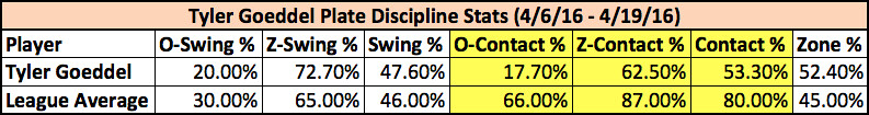
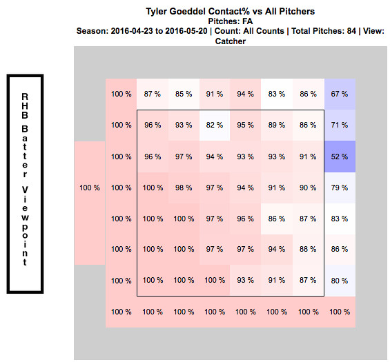
Overall, Martin’s plate discipline metrics show that his approach at the plate hasn’t changed too drastically from last season. If anything, his 70.4% contact rate is his lowest since 2012. One other thing sticks out here, namely that Martin seems to be more patient on pitches out of the zone and more aggressive on pitches in the zone. Compare the percentage of pitches he swings at in 2015 (left) to 2016 (right), courtesy of BrooksBaseball.net:

There is a relatively noticeable difference here, especially on high and outside pitches. According to PITCHf/x, his O-Swing% of 27.9 is easily the lowest of his career. Likewise, his Z-Swing% of 67.0 is his highest since 2012. These are generally good indicators that Martin is seeing the ball better or, at least, cut down on his tendency to chase pitches out of the zone.
And then there’s the matter of his batting stance.
Take a look at his stance for this home run on May 27, 2015, facing off against Scott Atchison:

Now check out his stance almost a year later, on May 22, 2016 in this at-bat against John Lamb.

An important thing to note about these stills is that I picked them mostly because of their similar camera angles. Martin’s foot position in other highlights is often obscured by the pitcher, or the pitcher is already in the middle of his wind-up, giving Martin time to square up before the pitcher’s delivery (as is slightly apparent in the at-bat against Lamb). But the vast majority of video evidence from this season is consistent with the idea that Martin has generally closed off his stance and now begins pretty much every at-bat with his feet squared to the pitcher. Now, I am aware that the batting stance is a rather fluid component of any baseball player’s oeuvre and can change for a number of reasons, not all of them being deliberately engineered to improve performance. I can’t seem to find anything about Martin having changed his stance online, aside from this ESPN piece from February of this year — but the focus of that article is on a legal issue Martin dealt with over the offseason, and the only comments offered on Martin’s approach seem to indicate that his stance hadn’t actually changed:
Martin also worked with a hitting instructor during the offseason in Miami. He altered his approach at the plate — his stance remains the same, he said — and he was pleased with the results when he faced pitchers in winter ball.
The most significant changes I’ve noticed as a result of comparing film from 2015 to film from 2016 are the aforementioned foot positioning and the fact that his hands are a little bit closer to his body this year. Generally speaking, though, it’s hard to really quantify the connection between a player’s stance and his performance. If this change in stance is deliberate, we can only really speculate as to the reasoning behind it. There are certainly good reasons to make the adjustments Martin has made. Bringing the hands closer to the body is often a nice starting point for a player who wants to make his swing a little more compact and less erratic. As for the foot positioning, there are a few benefits to batting with an open stance, especially for a left-handed hitter. One is that it enables left-handed hitters to see the ball better, especially when facing a left-handed pitcher. Another is that it eliminates the problem of the front foot stepping away from the plate on the swing, as batting from an open stance requires you to bring your front foot towards the plate in order to square up to hit the ball. It’s hard to say if Martin has previously had this issue in the past, but the fact that he’s changed from an open stance to a square stance likely indicates to me that whatever advantage he gained from an open stance may no longer be necessary. We don’t know if Martin has made these adjustments for the reasons listed above or if he has made them for any real reason at all, but he’s still made them all the same, and as it happens, they’ve been working out quite nicely for him.
That said, let’s not go overboard about a quarter-season of statistics just yet. Though Martin is posting career bests in almost any meaningful batting metric, there is still reason to believe he might still turn out to be an average or below-average hitter for the rest of the season. His on-base record is rather inflated by recent performances, he strikes out too much, and he continues to sport uninspiring numbers against left-handed pitching. All the same, his eight home runs this season aren’t going away, even if his fly-ball rate might. It’s unlikely, barring injury, that he’s not going to hit any more home runs for the rest of the year, so 2016 will most likely be a career year for him in the power department, and if his BABIP mark of .302 this year can regress back to his 2013-14 average of .326 rather than his poor 2015 mark of .270, 2016 may turn out to be a career year for him across the board. Martin’s offensive production has certainly been a pleasant surprise for the Mariners, and it would be interesting to know if altering his batting stance was a deliberate factor in producing an improved approach at the plate. If the Leonys Martin we’ve seen so far this year is anything like the Leonys Martin we’re going to see for the rest of the year, Jerry Dipoto may have stumbled upon a surprisingly high return on what was initially a low principal investment.