This article was co-authord by Daanish Mulla (@DanMMulla)

A New York Times article by John Branch in October 2015 discussed the elusive definition of the pitching term “stuff”. Talk of “plus stuff” and feelings of “all the stuff being there” was scattered throughout the article. Despite interesting commentary discussing the ability for pitchers to over-power hitters, there was no true definition of the nastiness of a pitcher’s stuff.

Earlier this November, Eno Sarris wrote an article examining who had the best changeup in the 2015 season. This was evaluated by looking at the difference in speed and movement with respect to the pitcher’s fastball. This made us think, to truly quantify “stuff”, you would first need to understand what goes into a pitcher having a truly dominant repertoire.

Our definition of a pitcher’s “stuff”, or their overall nastiness, was based on three different factors: 1) fastball velocity; 2) change of velocity of a secondary pitch with respect to the fastball; and 3) movement with respect to the fastball. We downloaded all of FanGraphs’ PITCHf/x data from 2008 to 2015 to attempt solving this problem.

For a pitch to qualify for this analysis, it had to be thrown by an individual pitcher at a frequency equal to, or greater than, the average frequency for that pitch to be thrown throughout the entire data set. For example, in our data set, the curveball was thrown at an average of 12% of the time by all pitchers. Thus, a pitcher’s curveball was only considered if it was thrown at a frequency of greater than or equal to 12%. We then determined the maximum and minimum velocity for all eligible pitches for each pitcher. Working off of the fastball, we then determined the maximum change in movement in both the X direction, and the Z direction, for any qualifying pitches. We then calculated the maximum resultant movement for these values. Z-scores were then calculated and summed from the following factors to get a final pitcher “stuff” score: 1) maximum velocity; 2) change in velocity between maximum and minimum velocity; and 3) maximum resultant movement.

Here is an example as to how a pitcher with elite stuff performed in this analysis. David Price had a great year with the Blue Jays and Tigers. From FanGraphs data, his maximum pitch velocity was 94.1 mph, and the minimum pitch velocity was 85.2 mph – a difference of 8.9 mph. Working off the fastball, the greatest x direction break on a pitch was 15.1”, and the greatest z direction break was 10.9”.  This produced a resultant change in movement of 18.6”.

These values translated to a z scores for velocity, change in velocity, and resultant movement of 0.969, -0.08, 0.91, resulting in a stuff value of 1.80. Comparatively, another Blue Jays starter who struggled in 2015 was Drew Hutchinson. Hutchison had a fastball velocity of 92.4 mph, an offspeed pitch of 84.3 mph, an x direction break of 7.1, and a z direction break of 9.8. Corresponding z scores for velocity, change in velocity, and resultant break were 0.392, -0.24, -0.08, resulting in a stuff value of 0.1.

To break down how well our stuff rating was performing, we correlated stuff with K/9. Pitchers included in this analysis were all starting pitchers who pitched 90 innings in a season, between the 2008 and 2015 season. Average stuff and average K/9 was calculated during this time. Overall, the correlation was r = 0.42 (Figure 1). For the sake of these graphs, knuckleballers Tim Wakefield and R.A. Dickey were not included, as the stuff metric had them rated lower than -4 per season.

View post on imgur.com

Figure 1. Stuff vs K/9, between the 2008 and 2015 MLB season.

Here’s the top 25 starting pitchers from the 2015 season ranked by their stuff. While overall, we think this is a good starting point for evaluating a pitcher’s repertoire, there are a few notable pitchers that the stuff calculation doesn’t seem to do justice. Chris Archer, who has had his slider called one of the best pitches in all of baseball, has only a 1.12 stuff value, and is ranked as having the 67^th best stuff. Max Scherzer, who threw two no-hitters, is ranked as only having the 60^th best stuff.

View post on imgur.com

Table 1. Top 25 stuff for pitchers, with raw data on velocity and break

What’s worth stressing however, is that this metric serves to evaluate the individual pitches within their repertoire. There are pitchers which would be scouted to have the ability to throw hard, with lots of break. Pitching is clearly an art form that involves more than those two things, thus players like Mark Buerhle (-2.7), are clearly someone who has mastered the art of pitching, without having great stuff.  When comparing stuff against xFIP, correlation coefficients are smaller (r = -0.33) (Figure 2). Much like K/9 does not directly predict pitcher success, neither does stuff.

View post on imgur.com

Figure 2. Stuff vs. xFIP, between the 2008 and 2015 season.

We believe there’s great use for this metric. We think this metric can provide insight into how stuff changes with age, how stuff changes after a pitcher is injured, and how it can let a coach know when a player has returned to pre-injury form, and how a pitcher’s consistency with their stuff relates to success. As with any ranking that appears on the FanGraphs website, we’re sure that there will be debate – however, we are looking forward to the input from the community into how we can improve this technique.

References

Branch, J. (2015). The Mysteries of Pitching, and All That ‘Stuff’. Posted online, October 3, 2015. http://www.nytimes.com/2015/10/04/sports/baseball/the-mysteries-of-pitching-and-all-that-stuff.html

Sarris, E. (2015). The Best Changeups of the Year by Shape and Speed. Posted online, November 9, 2015. http://www.fangraphs.com/blogs/the-best-changeups-of-the-year-by-shape-and-speed/

Before the season began, I wrote an article comparing the Vegas odds of each team winning the World Series to the projected standings according to Steamer. This is a look back at that comparison.

Using the Vegas odds of winning the World Series and the Steamer-projected standings, there were some strong plays on the board before the season began. Let’s look at each division, in chart form, starting with the NL West. The first table shows the Steamer pre-season projections. The second table shows the actual standings.

RDif=Run differential
RS/G=Runs scored per game
RA/G=Runs allowed per game
EXT W=Wins greater or fewer than Steamer projected

What I wrote then: It’s interesting that Vegas is really excited about the Padres, at least compared to the Rockies and Diamondbacks, who don’t project to be that much worse but who face significantly longer odds. With the Giants’ recent success, they are probably the best play here. Even if you don’t think they can beat out the Dodgers for the division, they’ve proven that they can make a run if they get into the playoffs as a wild card team. Of course, this is an odd-numbered year, so you might want to save your money and look elsewhere.

What actually happened: Steamer nailed the top of the division, picking both the Dodgers and Giants to win just one fewer game than they each did. The Diamondbacks and Padres were flipped, with the Diamondbacks winning five more games than projected and the Padres falling five games short. The Rockies came in way under. Vegas was right about the Dodgers being the favorites, with the Giants having the next-best odds, but the hype around the Padres at the beginning of the year proved to be unfounded and the Diamondbacks finished better than 120 to 1 odds would have predicted.

What I wrote then: The play here is the Pittsburgh Pirates. They are projected to be just a game off the division lead, but with odds at 30 to 1. In a world full of parity, every team in baseball would have a .500 record and 30 to 1 odds and there would be no supermodels. That would be a sad, sad, world. In this world, the Pirates are projected to be better than .500 and should have better odds than 30 to 1. Meanwhile, Vegas is excited about the Cubs, giving them 14 to 1 odds (they opened at 45 to 1). Some of you may remember that in Back to the Future, the Cubs won the 2015 World Series (in a 5-game sweep over Miami) after starting the year with 100 to 1 odds. This could be the Cubs’ year, McFly!

What actually happened: Steamer nailed the order of this division, right down to the gap between the top three teams and the bottom two. In the upper half of the NL Central, the Cardinals and Cubs shared the third-best odds in the National League and finished 1^st and 3^rd in overall win-loss record. The Pirates, on the other hand, finished with the second-best record in the NL but Vegas had them tied for eighth with the Marlins at 30 to 1 odds before the season. The Brewers and Reds both disappointed, but the Reds were particularly bad. They entered the season with 70 to 1 odds but finished the season with just 64 wins, one more than the Philadelphia Phillies, who were giving 300 to 1 odds back in April.

What I wrote then: There aren’t any real good plays here. As good as the Nationals look now, especially after acquiring Max Scherzer, it would be foolish to put any money on a major league team at 5 to 1 odds to win the World Series. There’s just too much unpredictability come playoff time. None of the teams in this division have appealing odds, unless your name is Lloyd Christmas, in which case you have to jump all over the Phillies at 300 to 1 (“So you’re telling me there’s a chance?”).

What actually happened: So much for those 5 to 1 odds in Vegas for the Washington Nationals. I hope you didn’t put too much money on them. Vegas was optimistic about the Nationals, as you would expect, but also gave the Marlins nearly the same odds as the Mets. The Mets made it all the way to the World Series, while the Marlins were 20 games under .500. The Phillies were the longest of longshots to win the World Series and finished with the worst record in the National League.

What I wrote then: There’s no love for the Tampa Bay Rays in Vegas, with odds of 75 to 1 in what still looks like a tight division. The Rays opened at 35 to 1. Apparently, Las Vegas does not like their recent moves. Based on Steamer projections, the Rays look like your best longshot option of any team in baseball.

What actually happened: At 14 to 1, the Red Sox were tied with the Seattle Mariners for the second-best odds of any American League team, with only the Los Angeles Angels topping them. The Red Sox (and Mariners) finished well below Steamer’s expectations. In the case of the Red Sox, the pitching didn’t hold up their end of the bargain. On the other hand, the Toronto Blue Jays had worse odds than nine other teams in the AL but finished with the second-best record in the league. They had nine more wins than Steamer projected.

What I wrote then: No team jumps out here, but if I had to pick one, I’d take the Indians at 25 to 1. They look to be right there with the Tigers to win the division, but with slightly worse odds, so you’d get a bigger payout if they went all the way.

What actually happened: I picked the Indians as the team to take a chance on, but everyone now knows the Royals were the best play. The 2015 World Champion Kansas City Royals were given 25 to 1 odds before the season started. Those odds placed the Royals behind six AL teams and tied with two others. They ended up with 14 more wins than projected by Steamer. The Tigers were the anti-Royals, finishing with 11 fewer wins than projected. The Tigers’ 20 to 1 odds were in the top six in the league and they finished with the second-worst record. The team with the longest odds in the AL, the Twins, actually made a run at a wild-card spot and had seven more wins than projected by Steamer.

What I wrote then: I guess when you lose Josh Donaldson, Brandon Moss, Jeff Samardzija, Jon Lester, and Derek Norris, your odds to win the World Series should get worse, but 60 to 1, really? Steamer still has Oakland in the mix for the AL Wild Card and just 5 games back of the Mariners for the division.

What actually happened: Based on their 68-94 record, the Athletics deserved their pre-season 60-to-1 odds, but they weren’t as bad as their record. They had a run differential that was better than the Mariners, who won eight more games than the A’s. The Angels (10 to 1), Red Sox (14 to 1), and Mariners (14 to 1) were the top three favorites in the AL in Vegas before the season started and they finished, 6^th, 11^th, and tied for 12^th, respectively, in wins. The Angels were within range of a wild card spot and actually had one more win than Steamer projected, but the Mariners were big disappointments in Vegas and compared to their Steamer projection. They had 13 fewer wins than Steamer projected. The 50 to 1 Rangers had the worst Vegas pre-season odds of any team that went on to win their division.

The following chart shows the teams in each league with their pre-season Vegas odds, their Steamer projected win-loss record, and their actual win-loss record.

What I wrote then: The Pirates have worse odds than the Padres and Mets, neither of whom are projected to contend for the Wild Card or even finish .500. Aye, this be the National League team you should wager your doubloons on and win some booty!

What actually happened: The Pirates weren’t a bad play, really. They did win 98 games. They just ran into the Jake Arrieta Experience in the one-game wild card matchup with the Cubs.

Based on pre-season Vegas odds, the top five teams in the National League were the Nationals, Dodgers, Cardinals, Cubs, and Giants. Three of those five made the post-season. Steamer, on the other hand, had a top five of the Nationals, Dodgers, Cardinals, Pirates, and Cubs, giving them four of the five post-season teams. Both Vegas and Steamer missed out on the Mets.

The Vegas pre-season odds did a good job of identifying the league’s worst teams. Five teams finished with fewer than 70 wins and they all had odds of 60 to 1 or worse before the season started. The 120 to 1 Diamondbacks were the exception among the teams expected to struggle in 2015, as they surprisingly won 79 games.

What I wrote then: In the American League, your best options are the Athletics and Rays, and possibly the Blue Jays. The A’s are right in the mix for the wild card, yet have the same odds as the Houston Astros and Atlanta Braves. The Rays are projected to be nearly as good as the A’s and have even worse odds, better than only four teams in all of baseball—the Phillies, Diamondbacks, Rockies, and Twins. The Blue Jays don’t look to be as good a play as the A’s and Rays but, like the Pirates, they have longer odds than other similarly competitive teams.

What actually happened: It turned out the A’s and Rays were not good plays, but how about those Blue Jays?

The Vegas pre-season odds suggested a top six of the Angels, Mariners, Red Sox, Tigers, Orioles, and White Sox, with all given odds of 20 to 1 or better. None of the six made the playoffs. You have to get down to the 25 to 1 Yankees and Royals to find a playoff team and they were joined by the 30 to 1 Blue Jays, 50 to 1 Rangers, and 60 to 1 Astros. Steamer projected a top seven that included the Mariners, Red Sox, Tigers, Angels, Indians, Blue Jays, and Athletics, all with 84 wins or more. Only the Blue Jays were a playoff team among this group.

The bottom line is that baseball is difficult to predict. Eleven teams had better odds than the World Series Champion Kansas City Royals and four teams had the same odds as the Royals. Yet, it was the Royals hoisting the World Series trophy when all was said and done.

With the World Series over and all the free agents declared it’s now time for my second-favorite part of the MLB season: the offseason. The 2015 free-agent class is pretty deep and includes some elite players. In this article I wanted to figure out a way to determine monetary value for the top three starting pitchers available this year: Zack Greinke, David Price and Johnny Cueto. All of them are aces and certainly heading for a big pay day but I wanted to develop a way of using the recent big contracts pitchers have signed and the production of great players in the past to determine what kind of pay day these guys are heading for.

Since 2009 there have been nine pitchers to sign a major deal: Clayton Kershaw, Max Scherzer, Justin Verlander, Felix Hernandez, C.C. Sabathia, Jon Lester, Zack Greinke, Cole Hamels and Matt Cain. (I didn’t include Masahiro Tanaka because he didn’t face big-league hitting until he signed his contract.) The average salary amount for these contracts was $168 million and had an average year length of about 5-6 years. When we’re looking at contracts there are many things to consider but two of the biggest factors has to be dollar and year amount. For all three of these pitchers, this may be their last big contract, so maximizing potential is crucial. Every team would love to add a pitcher of their caliber but not every team is in a position to pay for them. That’s part of the reason I wanted to figure out a way to see what dollar amount these pitchers’ production has warranted so far, in comparison to the big contracts signed since ’09 and speculate what can be expected of them for the length of the contract.

To figure out the dollar amount I looked at the nine players’ contracts and figured out the average yearly salary for each individual. I then took that number and divided it by their career WAR, essentially figuring how much it cost the team for the player’s WAR production. Here are the results I got (in millions).

Clayton Kershaw – $5.2m
Justin Verlander – $7m
Felix Hernandez – $6.5m
Jon Lester – $8.9m
C.C. Sabathia – $6.7m
Cole Hamels – $7m
Matt Cain – $9.4m
Zack Greinke – $7.7m
Max Scherzer – $7.5m

I averaged out the numbers, rounded off and got $7.3 million per WAR created. I then took that 7.3 number and multiplied it by Greinke’s career WAR to get, 27.7. So theoretically a year of Zack Greinke pitching is roughly $27.7 million. For David Price it’s $29.2 million and for Johnny Cueto it’s $21.1 million. It’s hard to predict where the market will go once teams start the bidding war, and I’m sure some team is willing to pay above the WAR value to ensure they get their man but for now I’m going to use these numbers to speculate year amount and production.

To determine the amount of years each player could receive, I decided to compare their career production with that of a similar type of pitcher. Let’s start with Zack Greinke. For Greinke I went with Greg Maddux as a comparison; obviously Greinke throws harder but I felt their command of the strike zone and pitches put Maddux and Greinke in the same boat. Below I’ve compared Greinke’s first 12 years in the big leagues to Maddux’s and I certainly think they’re close.

Zack Greinke      Greg Maddux

ERA = 3.49          ERA = 3.06
IP = 2,092.1         IP = 2,596.7
BABIP = .299       BABIP = .283
WAR = 3.8           WAR = 5.5
K/9 = 7.97            K/9 = 6.27
BB/9 = 2.37          BB/9 = 2.23
FIP = 3.52            FIP = 3.06
HR/9 = .92           HR/9 = .49

At age 32 Maddux had a better WAR than Greinke and threw about 500 more innings, but the latter may work in Greinke’s favor. The next part will help determine how many years a team can reasonably expect Greinke to pitch at an elite level. I looked at Maddux’s career numbers from age 32-38 and these were the results.

Greg Maddux (Age 32-38)

ERA = 3.21
IP = 1,581.6
BABIP = .285
WAR = 5.3
K/9 = 6.18
BB/9 = 1.50
FIP = 3.46
HR/9 = .81

As you can see from the results, Maddux was still pitching at an elite level from ages 32-38. From the ages of 39-41 however, you have a different story.

Greg Maddux (Age 39-41)

ERA = 4.20
IP = 827
BABIP = .291
WAR = 3.5
K/9 = 4.93
BB/9 = 1.39
FIP = 3.88
HR/9 = .91

Still good enough to be a major-league pitcher but a far cry from his prime. For Greinke’s situation I think you can expect a similar outcome, so a contract of 6 years at $166 million would be incredibly reasonable for a team. But this is America and money talks; whichever team is willing to pay the elite price tag for more then six years, I think, will be the winner of his services. A seven-year contract between $27-$29 million would be palatable and completely plausible but I think you start to handcuff yourself as a team going for eight years at that rate. Greinke had a dominant 2015 and if there ever was a time for him to test the open market, it’s now. We’ll see what teams are willing to shell out for him but for now let’s move on to David Price.

Unlike Greinke, David Price has never had a chance to test the open market and after another stellar season in the big leagues, Price is gearing up for a big pay day. As I mentioned before Price has a WAR value of about $29.2 million per season and at the age of 30 could see a lengthier contract then Greinke. To figure out future production I could only go with another tall, hard-throwing left-hander by the name of Randy Johnson. Price has eight years under his belt and his comparison to Randy Johnson looks something like this.

David Price          Randy Johnson

ERA = 3.02          ERA = 3.44
IP = 1,439.8         IP = 1,457.8
BABIP = .275       BABIP = .279
WAR = 4              WAR = 4
K/9 = 8.34            K/9 = 9.78
BB/9 = 2.43          BB/9 = 4.46
FIP = 3.30            FIP = 3.43
HR/9 = .80           HR/9 = .76

Price and Johnson compare very well, with Johnson having the advantage in K/9 but Price’s BB/9 is significantly better. Both have a WAR of 4 and nearly identical IP, BABIP, FIP and HR/9. Over the next eight years Johnson went on to be one of the most dominating pitchers in the game and during that stretch had some of the greatest seasons we’ve seen from a pitcher, period. Here are his numbers from 1996-2003.

Randy Johnson (’96-’03)

ERA = 2.93
IP = 1,660.8
BABIP = .308

WAR = 7
K/9 = 12.04
BB/9 = 2.79
FIP = 2.85
HR/9 = .94

This was by far the prime of Johnson’s career and although Price may not put up those types of numbers, he has a good shot of coming close. An 8-year deal for $233 million would be a steal if Price could come close to Johnson’s numbers. Price’s situation is similar to Greinke’s whereas whichever team is willing to pay elite prices for the most years will probably win out. Like Maddux, if you look at the back end of Johnson’s career, you’ll see the decline in results. Still effective for a major-league pitcher but not worth the elite money they once were.

Randy Johnson (’04-’09)

ERA = 4.00
IP = 1,011.6
BABIP = .290

WAR = 3.8
K/9 = 9.09
BB/9 = 2.21
FIP = 3.70
HR/9 = 1.21

Again, whichever team is willing to pay the elite price tag for these years of Price’s career will probably be the winner. It’s a gamble for sure to exceed eight years but eight elite seasons of David Price might be worth a year or two of mediocre Price. This brings us to our last top-tier starting pitcher and the one who perhaps stands to gain the most by being in the same class as Greinke and Price: Johnny Cueto.

First off, I want to say that I think Cueto is a great pitcher and one who deserves the “ace” title, and I know he’s spent most of his career in a hitter-friendly ballpark, but I don’t think his numbers warrant the price tag that Greinke and Price may receive. That being said, pitching is crucial for success in the big leagues and there are only a few top-tier pitchers available via free agency. A team that loses out on Greinke and Price could very well overpay for Cueto’s services to ensure they get one of the best available. For comparison I decided to use Jake Peavy; although Peavy is still playing I think his time as the ace for San Diego and his funky delivery pair nicely with Cueto. Here are the comparisons for the two pitchers through the first eight seasons of their careers.

Johnny Cueto          Jake Peavy

ERA = 3.31            ERA = 3.34
IP = 1,418.7           IP = 1,360.1
BABIP = .272         BABIP = .286
WAR = 2.9             WAR = 3.7
K/9 = 7.35              K/9 = 9.00
BB/9 = 2.65            BB/9 = 2.94
FIP = 3.87              FIP = 3.46
HR/9 = .94             HR/9 = .90

Through similar innings pitched Cueto and Peavy have comparable ERA, BABIP, WAR, BB/9, FIP and HR/9. The WAR value that I came up with for Cueto was $21.1 million per season, a number I think he can certainly get for a number of years. He’s only 29 and unlike Greinke and Price, may be able to sign two major contracts in his career if he can maintain elite status throughout the first one he is about to sign. If he were to sign a four- or five-year deal (4 years/$84 million or 5 years/$105), it’s not crazy to think that a team will pay the elite price tag for another three or four years of a quality Johnny Cueto.

The red flag I see with Cueto is the amount of innings he’s thrown; at 29 he’s only 21.1 innings away from David Price’s total of 1,439.8. As is the case with Jake Peavy, injuries completely derailed effectiveness and Peavy quickly went from “ace” to a 3rd or 4th starter. I’m not saying Cueto is destined to get hurt — his chances are the same as anyone, but paying the high price required to get him makes the possible injury sting even more. Here are the numbers Jake Peavy has put up over the past 6 seasons.

Jake Peavy (’10-’15)

ERA = 4.06
IP = 893.8
BABIP = .281
WAR = 2.3
K/9 = 7.39
BB/9 = 2.31
FIP = 3.82
HR/9 = 1.04

As I mentioned above, injuries greatly affected Peavy’s last six seasons and that’s not the best situation to compare future production from Cueto but it could be a caution to whichever team signs him as to the other end of the spectrum. We all hope for the best but you have to plan for the worst and shelling out $21m+ per season for those types of numbers doesn’t necessarily make sense.

Again I think Cueto is in a great position here, he’s young enough to sign a big deal and still have the potential to land another one down the road. It just depends on effectiveness and health; if both of those stay on his side, he should have no problem getting another big contract around 34 or 35.

After it’s all said and done, we’ll truly know the answer and that’s part of the fun. Speculating how much, how long and where players will end up helps get through the grueling winter months and I, for one, love it. Let me know what you think below and as always, thanks for reading.

In “Hardball Retrospective: Evaluating Scouting and Development Outcomes for the Modern-Era Franchises”, I placed every ballplayer in the modern era (from 1901-present) on their original team. Therefore, Rusty Staub is listed on the Astros roster for the duration of his career while the Athletics declare “Shoeless” Joe Jackson and the Blue Jays claim Tony Fernandez. I calculated revised standings for every season based entirely on the performance of each team’s “original” players. I discuss every team’s “original” players and seasons at length along with organizational performance with respect to the Amateur Draft (or First-Year Player Draft), amateur free agent signings and other methods of player acquisition.  Season standings, WAR and Win Shares totals for the “original” teams are compared against the “actual” team results to assess each franchise’s scouting, development and general management skills.

Expanding on my research for the book, the following series of articles will reveal the finest single-season rosters for every Major League organization based on overall rankings in OWAR and OWS along with the general managers and scouting directors that constructed the teams. “Hardball Retrospective” is available in digital format on Amazon, Barnes and Noble, GooglePlay, iTunes and KoboBooks. The paperback edition is available on Amazon, Barnes and Noble and CreateSpace. Supplemental Statistics, Charts and Graphs along with a discussion forum are offered at TuataraSoftware.com.

Don Daglow (Intellivision World Series Major League Baseball, Earl Weaver Baseball, Tony LaRussa Baseball) contributed the foreword for Hardball Retrospective. The foreword and preview of my book are accessible here.

Terminology

OWAR – Wins Above Replacement for players on “original” teams

OWS – Win Shares for players on “original” teams

OPW% – Pythagorean Won-Loss record for the “original” teams

Assessment

The 1907 Philadelphia Phillies    OWAR: 56.2     OWS: 349     OPW%: .527

Based on the revised standings the “Original” 1907 Phillies finished in a tie for fourth place, only six games behind the front-running Cubbies. Philadelphia paced the National League in OWS and OWAR.

Sherry Magee batted .328 with a League-best 85 RBI and a team-leading 37 Win Shares. Elmer Flick supplied a .302 BA and legged out 18 three-base hits. Nap Lajoie rapped 30 doubles and pilfered 24 bases. The keystone combo of Ed Abbaticchio and Kid Elberfeld swiped 57 bags. Roy A. Thomas posted a .374 OBP and led the League in walks for the seventh time in eight seasons. “Silent” John Titus provided a solid option as a fourth outfielder, belting 23 doubles and 12 triples while hitting at a .275 clip.

Nap Lajoie places sixth among second basemen according to Bill James in “The New Bill James Historical Baseball Abstract.” Teammates listed in the “NBJHBA” top 100 rankings include Magee (21^st-LF), Flick (23^rd-RF), Thomas (29^th-CF), Kid Gleason (72^nd-2B), Elberfeld (75^th-SS) and John Titus (76^th-RF).

Doc White fashioned a 2.26 ERA and a 1.058 WHIP while topping the leader boards with a 27-13 record. Tully Sparks delivered a 22-8 mark with a 2.00 ERA and 1.026 WHIP as he completed 24 of 31 starts. Johnny Lush (10-15, 2.68) and “Smiling” Al Orth (14-21, 2.61) rounded out the Phillies’ rotation. George McQuillan (4-0, 0.66) yielded only three earned runs in 41 innings pitched during his inaugural campaign.

The “Original” 1907 Philadelphia Phillies roster

Honorable Mention

The “Original” 1978 Phillies   OWAR: 57.7     OWS: 320     OPW%: .547

Clashing with the Expos and the Bucs into the final week of the ’78 season, Philadelphia emerged in third place, only two games behind Pittsburgh. The Fightin’ Phillies led the circuit in OWAR and placed runner-up to the Pirates in OWS. Greg “The Bull” Luzinski launched 35 moon-shots and knocked in 101 baserunners. First-sacker Andre Thornton blasted 33 long balls, tallied 105 RBI and scored a personal-best 97 runs. Larry Hisle delivered a .290 BA with career-bests in home runs (34) and RBI (115). Mike Schmidt struggled through a sub-par season at the dish but played stellar defensive at the hot corner, winning his third of nine consecutive Gold Glove Awards. Shortstop Larry Bowa contributed 27 steals and a .294 BA while backstop John “Bad Dude” Stearns pilfered 25 bases. Fergie “Fly” Jenkins furnished a record of 18-8 with a 3.04 ERA and 1.080 WHIP. Dick Ruthven provided 15 wins with a 3.38 ERA. Mike G. Marshall anchored the relief corps with 10 victories and 21 saves.

On Deck

The “Original” 2001 Mariners

References and Resources

Baseball America – Executive Database

Baseball-Reference

James, Bill. The New Bill James Historical Baseball Abstract. New York, NY.: The Free Press, 2001. Print.

James, Bill, with Jim Henzler. Win Shares. Morton Grove, Ill.: STATS, 2002. Print.

Retrosheet – Transactions Database

Seamheads – Baseball Gauge

Sean Lahman Baseball Archive

We could easily call my decision to publish an article with playoff predictions using a brand-new theory about previous success predicting future success ballsy (or stupid). To summarize, research by Rosenqvist and Skans (2015) [1] showed that golfers who barely qualified for a golf tournament would go on to have more success in future tournaments than golfers who barely missed the cut in the same tournament. Seemingly accidental success created confidence, which led to more success in the future. So, using this logic, I wanted to see if this same phenomenon occurred at the team, rather than the individual level. The attempt was to predict all divisional victors from this year’s 2015 MLB playoffs using previous playoff experience and success as the predictor. As it turns out, the teams with more experience/success were only 1 for 4 in the first round of the playoffs.

This time, instead of making predictions, I did the smart thing and looked at previous trends. Instead of using the first round of the playoffs (which arguably is more erratic given that it’s only a five-game series), I focused solely on the World Series. I totaled all the previous playoff experience, age, and WAR for every player on each 25-man World Series team roster in the Wild Card Era (1995 – 2015, n = 42 teams).

WAR doesn’t predict the winner of the World Series

Is this old news? I don’t know. Tallying up a team’s WAR correlates with the actual number of wins that team will have by the end of the regular season (somewhere around r = .82 last time I checked), but it doesn’t correlate with the victor of the World Series. In fact, 13 out of the last 21 (62%) World Series victors had average WARs lower than their opponent’s.

Differences in experience at the team level relate to the duration of the World Series

The difference in previous playoff experience between the two World Series teams is a good predictor of the number of World Series games that will be played in a series. Specifically, at the team level, the greater the difference in the average previous playoff series won (r = -.45, p < .05, n =21), the average number of World Series appearances (r= -.45, p < .05, n =21), and the average number of World Series titles (r = -.46, p < .05, n =21) between the two teams, the less World Series games played that year. You’re saying, “yeah but what about the 2014 World Series that went 7 games when the seasoned Giants played the inexperienced Royals?” It’s just a trend, not a guarantee.

Other tidbits

• The higher the average of previous World Series appearances across both World Series teams, the higher number of television viewers (r = .45, p < .05).
• The World Series victor with the highest average WAR per player was the 1998 Yankees (m = 2.57); the lowest WAR was the 2006 Cardinals (m = 1.26).
• Oldest World Series victors were the 2000 Yankees (m = 30.7); youngest were the 2002 Angels (m = 27.4).
• Most experienced victor was also the 2000 Yankees (96% of the team had previous playoff experience), and least experienced were the 2002 Angels (0%).

More needs to be understood about this theory

There was however, no relationship between previous playoff experience and that year’s World Series outcome. In terms of playoff experience, the results from Rosenqvist and Skans could not be replicated in this setting. Baseball isn’t golf, and baseball isn’t an individual sport, it’s a team sport. Perhaps the average and/or aggregate levels of experience within a team might manifest differently than for an individual. So, too, are there other ways to operationalize this hypothesis of previous experience/success, so I wouldn’t write this off as a done deal. We’re still a long ways away from determining how and if this theory occurs within the context of baseball – more research into the theoretical underpinnings is always the answer.

Back to the drawing board.

[1] Rosenqvist, O. & Skans O.N. (2015). Confidence enhanced performance? – The causal effects of success on future performance in professional golf tournaments. Journal of Economic Behavior & Organization, 117, 281-295.

This increasing time of games has been cited by Major League Baseball to be a deterrent to fans, jeopardizing ticket sales. Total game time has increased between 2.85 hours in 2004, rising to 3.13 hours in 2014. In 2015, MLB implemented rules to help speed up game time. These rules included forcing batters to stay in the batter’s box during at-bats, and decreasing the time between innings to 2 minutes and 30 seconds. Back in April, after the first few weeks of the season had passed, MLB reported success on their initiatives, stating that if current paces were maintained, average game time would drop below the 2.92-hour mark for the first time since 2011.

A more dramatic possible change was to implement a pitch clock, forcing pitchers to throw their next pitch within 20 seconds of receiving the ball back from the catcher. Currently, the rulebook states (Rule 8.04) that pitchers should throw their next pitch within 12 seconds of receiving the ball from the catcher. However, this rule is not enforced. FanGraphs presents data on the time between pitches, called Pace, which is calculated by taking the total time in an at-bat, and dividing it by the number of total pitches. Between 2010 and 2014 (for pitchers who threw at least 50 MLB innings), the slowest pitchers were Jose Valverde in 2012 (32.4 seconds), Joel Peralta in 2012 (32.3 seconds), and Joel Peralta in 2014 (32.1 seconds). The fastest pitchers were Mark Buehrle in 2010 (16.4 seconds), Mark Buehrle in 2011 (15.9 seconds), and (drum roll please… ) Mark Buehrle in 2015 (15.9 seconds). However, what goes into a pitcher’s selected pace? Focus on execution of their pitch? Embracing the glow of the national spotlight? There hasn’t been much (if anything) to describe the relationship between a pitcher’s self-selected pace and pitching performance.

I looked at the average pace for all pitchers who threw a minimum of 50 innings in years 2010 through 2015. The time between pitches increased steadily between 2010 and 2014, rising from 21.9 seconds in 2010, to 23.5 seconds in 2014. In 2015, the influence of the new pace-of-play initiatives could be seen, with pace decreasing to an average of 22.2 seconds between pitch. Definitely a step in the right direction from MLB’s perspective, but how did this impact pitching performance?

Focusing on xFIP for all pitchers from the same cohort (a minimum of 50 IP), a trend existed for xFIP to decrease between years 2010 and 2014 – an inverse relationship compared to pitching pace. In 2010, the average xFIP was 3.98, compared to 3.60 in 2014. In 2015, xFIP increased to 3.84.

View post on imgur.com

Is this truly a reflection of pitchers requiring an extra second or two to steady themselves and prepare to throw their best possible pitch in a given situation – or are other factors in play? From a physiological perspective, reducing the time between physical efforts can result in an increased accumulation of muscle fatigue. A recent paper published in the journal of Sports Sciences by Wang and colleagues (2015) found pitchers in a fatigued state were less able to throw strikes. A possible explanation of this relationship is found between increased pitching pace and decreased xFIP.

Major League Baseball will surely press forward with what is best for the game, and the business of baseball. It would be worthwhile for coaches, pitchers, and player’s union representatives to further investigate how pitchers self-select their pace between pitches. Further work is required to establish if there are any negative health consequences associated with decreasing the time between pitches. This should be completely ruled out before any further initiatives are taken by the MLB to speed up the game of baseball.

References

Every athlete, professional or otherwise, talks about that feeling of being on a team. There’s something that happens when a team “clicks” – it’s a united feeling of team spirit that propels team members to compete, most often referred to as team chemistry. In the social sciences there’s no measure of team chemistry, but there is however Team Cohesion, which is defined as:

A dynamic process that is reflected in the tendency of a group to stick

together and remain untied in the pursuit of its instrumental objectives

and/or for the satisfaction of member affective needs [1].

Team cohesion has been shown to exist across multiple work group settings (organizational, military and sport) [2], as well as across multiple sports (basketball, golf [3], softball, and baseball [4]). Perhaps more interestingly, cohesion has also been bi-directionally linked to performance: when teams perform better, they are more cohesive; and when they are more cohesive, they perform better [2,5]. And while the research on this relationship is clear, it has mostly been conducted with non-professional teams. Indeed, team cohesion is one of many other “unobservable” properties that are untapped within profession sports.

How can we measure team cohesion in professional sports?

 As researchers, we would normally use a validated survey to measure team cohesion – a survey that I could rely on to accurately measure team cohesion. Unfortunately, when I don’t have access to a team, I’m forced to use alternative methods. The first step is to examine the literature; a few key findings are brought to light about indications of team cohesion:

• Team cohesion is related to the extent that members accept the roles on their team (captain, motivator, leader, follower, etc.) [6].
• Charismatic leaders will refer to their teams more often than referring to themselves [7].
• The higher the level of team cohesion, the better the team performance [2,5].

So, if I can somehow measure how often leaders refer to their teams (vs. themselves), then I can use this as an approximation of their leadership characteristics. And if leaders are acting like leaders, they may also be helping to solidify roles within their team. Therefore we might expect that:

Hypothesis 1: As leaders reference their team more, we should see increased team cohesion – and as team cohesion increases, we should see better performance.

A charismatic leader does not typically arise without a contextual or conditional trigger. Crisis often prompts the emergence of charismatic leadership – a setting that allows a charismatic leader to propose an ambitious goal [8]. Both the context and the charismatic leader influence one another, almost as if the leader requires crisis as an occasion to exemplify charismatic leadership [9]. Additionally, at the group level, team members have been shown to become more attached to the leader in times of crisis, prompting a greater presence of cohesion during times of crisis as followers rally around the charismatic leader [10].

In baseball, teams experience all types of crises throughout the long season, including injuries, losing streaks, playoff races, and team conflicts. Perhaps the most common and least contextual of these crisis is the race to the playoffs as the season comes to an end. With an understanding of how and when the playoff races begin to make an impression, I can expect to observe a temporal effect of charismatic leadership by using our previous indicator of team reference. That is, it may not only be that “there is a positive relationship between a leader’s team references and the amount of wins his team will have at the end of the regular season”, but also:

Hypothesis 2: The timing of when a team leader references his team can determine the effectiveness of his leadership.

Methods

As the first component of the measure, I needed to assess team leaders’ reference to themselves or their team, I used the most popular newspaper from that team’s city to extract quotations (e.g., San Francisco Chronicle for the Giants; the New York Times for the Yankees). A team leader was identified by teammates, coaches, or front offices as a “leader”, a “captain”, or having either of these qualities. If there was more than one identified team leader, I randomly chose between the two. I tracked the quotes from 8 randomly selected baseball team leaders from 8 randomly selected teams across an entire regular season (April 4^th, 2012 – October 3^rd, 2012). Statement settings included comments made in locker rooms after games, during the All-Star break, before a game started, or in any other setting. Any time the leader was documented as saying anything that appeared in the newspaper, that quote was documented for analysis. Leader quotes were qualitative coded independently between 3 different coders. Each quote was coded as containing “self-reference”, “team-reference”, and/or “other reference” (the 3 coders had 97% agreement on their final codes). I began this study in 2013 thus I used the 2012 season, which was the latest complete season at my disposal.

Due to the disparity in responses, the sample was aggregated based on team leaders who played on teams that finished with a certain number of wins. Since 1996, no AL team has made the playoffs with less than 86 wins [11]. During the same time period, no NL team has made the playoffs with less than 82 wins [12]. For this study, leaders were categorized based on how their teams finished the regular season (86 or more wins for AL teams and 82 or more wins for NL teams). Those at or above the win mark were titled “high team leader” (HTL) and those below the win mark were titled “low team leader” (LTL). Four teams in the sample met the HTL criteria and their combined record was 368 – 280 (.568 wining percentage). Not all HTLs were on teams that made the playoffs in 2012, but each of the four teams were competing for a playoff spot in the months of August and September. Four teams in the sample met the LTL criteria and their combined record was 296 – 352 (.457 winning percentage).

     Table 1. Classification of high or low team leaders based on their team’s 2012 regular season record

Results

There was no significant correlation between the total number of team references and the total number of wins that a leader’s team had at the end of the regular season r = .237, p > .05). Nor was there an indication of a negative correlation between self-references and total number of team wins r = -.086, p > .05.

Leader responses were then aggregated between LTLs and HTLs. Of the 490 total responses, 252 responses were made after or in reference to a previous game. Quotes were then selected for these post-game interview responses after a leader’s team had won a game (162 total) or lost a game (90 total). After a loss, both HTLs and LTLs referred to their teams much more often than referring to themselves. LTLs were 7.20 times as likely to reference their team after a loss than reference themselves. When compared to LTLs, HTLs were less likely to refer to their team after loss (4.42:1). After a win, LTLs were 1.41 times as likely to reference their team than themselves. HTLs on the other hand were 2.32 times as likely to reference their team than themselves after a win (Table 1).

     Table 2. Ratios of team vs. self references for each type of leader

The monthly distribution of team reference for LTLs was relatively even across all months of the regular season. The highest percentage was July (19.9%) and the lowest was August (12%), a difference of 7.9% (Figure 1). The overall standard deviation for team references by month was σ = 2.88. In contrast, team reference for HTLs was much more dynamic. The highest percentage was September (39.6%) and the lowest was June (5.8%), a difference of 33.8%. September team references for HTLs were more than double any other month. The overall standard deviation was σ = 12.2, with the resulting distribution becoming much more parabolic (Figure 2). The quadric trend line that is used to represent the team reference distribution for HTLs showed a very good fit R² = .91.

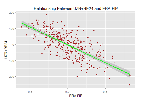
Figure 1. Percentage of team reference by month LTLs

           Figure 2. Percentage of team reference by month HTLs with quadratic trend line

Discussion

The increased rate of team reference by HTLs as compared to LTLs may have helped to establish better role clarity – a characteristic of more cohesive teams. This was further marked by the fact that HTLs were on higher performing teams than LTLs. The direction of the team cohesion to performance relationship in this case is still unknown.

HTLs also referred to their teams most often during the end of the regular season. This relates to the theory that charismatic leaders will “activate” in times of crisis. In turn, this helps to create more team cohesion as members attach themselves to leaders in times of crisis.

[1] Carron, A.V., Colman, M.M., Wheeler, J., & Stevens D. (2002). Cohesion and Performance in Sport: A Meta Analysis. Journal of Sport & Exercise Psychology, 24, 168-188.

[2] Mullen, B. and Copper, C. (1994). The relation between group cohesiveness and performance: an integration. Psychological Bulletin.115, 210-227.

[3] Vincer, D., & Loughead, T.M. (2010). The Relationship Among Athlete Leadership Behaviors and Cohesion in Team Sports. The Sport Psychologist, 24, 448-467.

[4] Carron, A.V., Bray, S.R., & Eys, M.A. (2002). Team Cohesion and Team Success in Sport. Journal of Sports Sciences. 20(2). 119-126.

[5] Oliver, L.W., Harman, J., Hoover, E., Hayes, S.M., & Pandhi, N.A. (2003) A quantitative integration of the military cohesion literature. Military Psychology, 11, 57-83.

[6] Carron, A. V., & Eys, M. A. (2012). Group dynamics in sport (4th ed.). Morgantown, Fitness Information Technology.

[7] Shamir, B., Arthur, M.B., & House, R.J. (1994). The rhetoric or charismatic leadership: A theoretical extension, a case study, and implications for research. The Leadership Quarterly, 5(1), 25-42.

[8] Poon, J. & Fatt, T. (2000). Charismatic Leadership. Equal Opportunities International. 19(8), 24-28.

[9] Conger, J. A. (1999). Charismatic and transformational leadership in organizations: An insider’s perspective on these developing streams of research. The Leadership Quarterly, 10, 145-179.

[10] Kets de Vries, F. R. (1988). Prisoners of leadership. Human Relations, 41, 261-280.

[11] Gaines, C. (2011, April 21). Chart of the Day: What it takes to make the playoffs in Baseball. Business Insider. Retrieved from http://www.businessinsider.com/chart-of-the-day- what-it-takes-to-make-the-playoffs-in-baseball-2011-4

[12] Bloom, B.M. (2005). Padres Try to Recover from 82-80 Record. San Diego Padres. Retrieved from http://m.padres.mlb.com/news/article/1236830/

In “Hardball Retrospective: Evaluating Scouting and Development Outcomes for the Modern-Era Franchises”, I placed every ballplayer in the modern era (from 1901-present) on their original team. Therefore, Frank Tanana is listed on the Angels roster for the duration of his career while the White Sox declare Edd Roush and the Yankees claim Hippo Vaughn. I calculated revised standings for every season based entirely on the performance of each team’s “original” players. I discuss every team’s “original” players and seasons at length along with organizational performance with respect to the Amateur Draft (or First-Year Player Draft), amateur free agent signings and other methods of player acquisition.  Season standings, WAR and Win Shares totals for the “original” teams are compared against the “actual” team results to assess each franchise’s scouting, development and general management skills.

Expanding on my research for the book, the following series of articles will reveal the finest single-season rosters for every Major League organization based on overall rankings in OWAR and OWS along with the general managers and scouting directors that constructed the teams. “Hardball Retrospective” is available in digital format on Amazon, Barnes and Noble, GooglePlay, iTunes and KoboBooks. The paperback edition is available on Amazon, Barnes and Noble and CreateSpace. Supplemental Statistics, Charts and Graphs along with a discussion forum are offered at TuataraSoftware.com.

Don Daglow (Intellivision World Series Major League Baseball, Earl Weaver Baseball, Tony LaRussa Baseball) contributed the foreword for Hardball Retrospective. The foreword and preview of my book are accessible here.

Terminology

OWAR – Wins Above Replacement for players on “original” teams

OWS – Win Shares for players on “original” teams

OPW% – Pythagorean Won-Loss record for the “original” teams

Assessment

The 1931 Philadelphia Athletics    OWAR: 53.6     OWS: 347     OPW%: .524

Connie Mack acquired all of the ballplayers on the 1931 Athletics roster. Based on the revised standings the “Original” 1931 A’s finished in second place, two games behind the Yankees. Philadelphia paced the Junior Circuit in OWS and led the League in OWAR for the fourth straight season (1928-1931).

“Bucketfoot” Al Simmons (.390/22/128) collected his second successive batting title and placed third in the American League MVP balloting. Mickey Cochrane drilled 31 doubles and delivered a .349 BA. Max “Camera Eye” Bishop amassed over 100 bases on balls in eight consecutive seasons (1926-1933). Jimmie Foxx belted 30 round-trippers and drove in 120 baserunners. Charlie Grimm aka “Jolly Cholly” contributed a .331 BA with 33 doubles and 11 triples.

Jimmie Foxx ranks second to Lou Gehrig among first basemen while Lefty Grove places runner-up to Walter Johnson according to Bill James in “The New Bill James Historical Baseball Abstract.” Teammates cataloged in the “NBJHBA” top 100 rankings include Cochrane (4th-C), Simmons (7th-LF), Wally Schang (20th-C), Bishop (43rd-2B), Jimmie Dykes (52nd-3B), Grimm (85th-1B), Joe Dugan (88th-3B) and Doc Cramer (91st-CF).

Lefty Grove claimed the 1931 American League MVP award with a dominant performance including League-bests in victories (31), ERA (2.06), WHIP (1.077) and complete games (27). He also struck out the most batsmen in the circuit for the seventh year in a row. George “Moose” Earnshaw topped the 20-win plateau for the third straight season. Herb Pennock and Tom Zachary furnished 11 victories apiece.

The “Original” 1931 Philadelphia Athletics roster

Honorable Mention

The “Original” 1911 Athletics            OWAR: 46.1     OWS: 303     OPW%: .597

Philadelphia coasted to the pennant by a nine-game margin over Boston. “Shoeless” Joe Jackson posted a .408 BA in his first full season. He collected 233 safeties, scored 126 runs and led the Junior Circuit with a .468 OBP. Eddie Collins swiped 38 bags while batting at a .365 clip. “Home Run” Baker (.334/11/115) topped the American League in circuit clouts for the first of four consecutive campaigns. Matty McIntyre totaled 102 runs and produced a .323 BA. “Gettysburg” Eddie Plank delivered a 23-8 record with a 2.10 ERA including six shutouts. Jack Coombs led the League with 28 victories despite allowing 360 hits in 336.2 innings pitched. Bris Lord aka the “Human Eyeball” supplied a .310 BA and accrued 92 tallies.

The “Original” 2002 Athletics            OWAR: 45.8     OWS: 304     OPW%: .578

Jason Giambi (.314/41/122) coaxed 109 bases on balls and tallied 120 runs as the ’02 squad finished five games ahead of the Angels for the American League pennant. Miguel Tejada (.308/34/131) achieved MVP honors and made his first All-Star appearance while registering 108 aces and 204 base knocks. Barry Zito claimed the Cy Young Award with a record of 23-5 and an ERA of 2.75. Tim Hudson contributed 15 victories and a 2.98 ERA while portsider Mark Mulder accrued 19 wins. Eric Chavez launched 34 long balls, drove in 109 baserunners and earned the second of six consecutive Gold Glove Awards.

On Deck

The “Original” 1907 Phillies

References and Resources

Baseball America – Executive Database

Baseball-Reference

James, Bill. The New Bill James Historical Baseball Abstract. New York, NY.: The Free Press, 2001. Print.

James, Bill, with Jim Henzler. Win Shares. Morton Grove, Ill.: STATS, 2002. Print.

Retrosheet – Transactions Database

Seamheads – Baseball Gauge

Sean Lahman Baseball Archive

It is well established that having more rise on your four-seam fastball is a good thing. The question then becomes, can we identify the optimal amount of rise as compared to the league-average fastball. For the purposes of this analysis, we will look at swinging-strike rate, from all four-seam fastballs thrown since the dawn of the PITCHf/x era, in regular-season action.

We in the sabermetrically-inclined community tend to pooh-pooh popular baseball concepts, particularly ones where the science, on the surface, doesn’t appear to jive with the age-old baseball wisdom. Don’t worry, this is not a DIPS discussion, nor a discussion on a pitcher’s ability to manage contact. I bring up this concept in relation to the term “late life” as in movement later in the pitches trajectory. Physics tell us that the ball will have a very predictable trajectory from the moment the ball leaves the pitchers hand, until it reaches the front of the plate. That, however, is merely half the story. There are two important points I want to bring up:

1. Batters cannot compute vertical trajectory explicitly; they essentially tap into a huge vault of experience telling them how far a pitch will drop based on their experience with pitches of similar velocity.
2. A hitter’s swing is largely ballistic (very difficult to change mid-swing) and takes about 0.18 seconds to execute. That means that a hitter has roughly 0.2 seconds post-release of the ball to gather information and form an educated guess as to where the ball will end up.

Based on these assumptions, I computed late movement, in both the vertical direction and horizontal direction. I then compared this to the expected vertical movement based on the velocity (more velocity, less drop obviously). This to me is the optimal way to look at movement, since presumably they cannot gather any more information. A great hitter may be able to factor in their knowledge of the pitcher’s ability to rise the fastball, but they are fighting their memories of all the other fastballs they’ve seen, so more difficult than you would think.

Which brings us to a very interesting graph: The height and colours in the histogram reflect the magnitude of the swinging-strike rates, shown in sequential order of velocity. If you scroll all the way to the bottom, you’ll see that the center of the histogram is somewhere around -.6, or 0.6 feet more rise than the average four-seam fastball when looking at the pitch 0.2 seconds after release until it crosses home plate.

We see a very clear normal curve, with more “normal” at higher n. Thus we can now compute the value of rise in a four-seam fastball, as distributed by a normal curve centered around 0.6 feet above the mean drop. Not really a stats guy, so not sure how to do that exactly. What I find interesting is that the 7 inches or so of rise is pretty consistent across the velocity spectrum. I’m not sure why it peaks at this point, though I would surmise that it’s probably the sweet spot where the hitter feels like they can make contact, but can’t, as opposed to extreme rise which would freeze the hitter.

This leads us to our last graph (warning: this one scrolls for a while). You’ll see the same graph as above, but you’ll see Whiff%, GB% and HR% stacked one on top of the other.

This actually paints a very intuitive picture. If there is more rise than average, you’ll get swinging strikes. If it drops more than average, you’ll get groundballs and if it drops about what you’d expect, you’ll get some groundballs, but also homers. Ignore the SSS noise with homers at the higher velocities. Again what is interesting with the GB% and Whiff% histograms are how consistent they are irrespective of velocity. So… if velocity doesn’t impact this analysis, let’s collapse it all into one final graph:

Paints a very clear picture: if your four-seam fastball isn’t getting at least 5 inches of late rise, you are going to be giving up a lot of homers. Note that swing% (swings/total pitches) is normally distributed around a mean of .2 feet of rise and appears to track pretty closely to HR%, implying that hard contact is not affected within 1 standard deviation.

Looking forward to the feedback.

References

Lin-Hwa Wang, Kuo-Cheng Lo, I-Ming Jou, Li-Chieh Kuo, Ta-Wei Tai & Fong- Chin Su (2015): The effects of forearm fatigue on baseball fastball pitching, with implications about elbow injury, Journal of Sports Sciences, DOI: 10.1080/02640414.2015.1101481
Measuring Team Chemistry with Social Science Theory