Archive for Uncategorized

Blast Motion Sensor: Correlation to On-Field Performance and How to Utilize it

Introduction

Athletes are always looking for an edge – how to get better, how to raise their level of play – and are looking for different tools and resources to help them to accomplish this goal. In recent years, baseball has been going through a boom of data-driven player development, with players and coaches looking for the best technology to increase on-field performance as much as possible. Technology allows for coaches to stop guessing, and instead to leverage data in order to deliver answers. As just one example, swing sensors have become extremely popular in recent years in both baseball and softball to help create better hitters.

The Blast Motion sensor, when attached to the end of the bat, gives the hitter different metrics pertaining to the swing. The Blast Motion sensor is the official bet sensor of Major League Baseball. As a baseball player looking for a data-driven way to objectively look at my swing and try to improve it, I purchased a Blast sensor last May. While using the sensor two important questions came up: (i) what metrics matter the most in creating the best possible swing? (ii) do any of these metrics correlate to on-field success? If this question can be answered, users of the Blast Motion sensor can be better prepared for how they use it to create better swings, and hitters.

There appear to have been no empirical studies of these questions, and so I decided to try to answer them myself.  I had an entire college baseball team full of hitters to use as my sample. My goal was to create a study looking into the metrics on the Blast Motion sensor and see which correlate the best to on-field success and therefore are the most important to focus on and gear your training towards.

Data Collection and Exploration

The sample of this study is the Babson College Varsity baseball team. Each member of the team took 50 swings using the Blast Motion Sensor on their bat over the course of a single batting practice session sometime between November 2017 and February 2018. Each player was given the opportunity to warm up before swinging to ensure they were loose and were swinging as hard as they could, just as happens in real games.  The swings were taken against an underhand toss that I threw. Having players hit against front toss rather than swing off a tee more closely simulates an in-game scenario. The 50 swings each player recorded were taken in 5 rounds of 10 swings. Players took a short break in between each round of 10 swings.

Gaining a better understanding of each metric provided by the Blast sensor will help me comprehend and analyze the conclusions I gather later on in the study. The definitions and calculations for each metric are detailed in the table below.

Metric Measurement Definition
Bat Speed (BS) MPH The speed of the bat at contact.
Attack Angle (AA) degrees The angle of the bat at contact where a completely flat-bat that is parallel to the ground is 0 degrees. If the bat is coming from a down-to-up angle that is positive and an up-to-down angle that is negative
Time to Contact (TTC) seconds The time it takes for a hitter to make contact with the ball from the start of their swing.
Peak Bat Speed (PBS) MPH The fastest speed observed at any point in the swing.
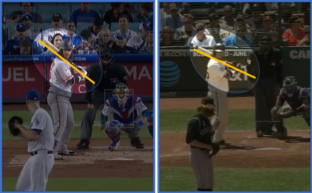
Vertical Bat Angle (VBA) degrees Vertical bat angle is the angle of the bat at contact with 0 degrees being a perfectly flat and horizontal barrel. A barrel that is below the hands at contact results in a negative angle(9). The ideal vertical bat angle range is -25 to -35 degrees (3) Figure 1 below displays Mike Trout making contact and is a good visual of where vertical bat angle is measured.
Power (P) kW Power is a measurement incorporating both bat mass and bat velocity. The average power generated during the swing is found from the effective mass of the bat, bat speed at impact, and the average acceleration during the downswing (10). Players with the ability to swing a heavier bat that they can accelerate faster produce more power.
Blast Factor (BF) 1-100 This is a metric created by the Blast team that is on the scale of 0-100 where 0 is the worst possible score and 100 is the best possible score. The 100 possible points in the blast factor are comprised of two equally weighted components: power and swing efficiency (1). The power part of it is comprised of the power metric. The efficiency part of Blast Factor is more complicated, and we will discuss it in more depth below.
Body Rotation (BR) 0%-100% Body Rotation is also rated on a 0-100% scale. Body rotation is expressed as the ratio of Body rotation during the time a players “wrists unhinge” to the total rotation during this time. (8). The ideal number for body rotation is 45% and ideal range is 40%-50%. .
On Plane Percentage (OPP) 0%-100% This metric calculates how “on plane” a player is. It is on a 0%-100% scale. The red line in figure 2 below represents the pitch plane. The green dots represent different points of Miguel Cabrera’s swing. The two dots that are roughly on the line represent the “on plane” portion of Cabrera’s swing. How well a player does this is represented in OPP. Blast calculates OPP by defining how long the sweet spot of a players barrel is on plane. The percentage is calculated by how well a players bat speeds up during this point (11).  A typical range for a good swing is 55%-65% (4).
Peak Hand Speed (PHS) MPH The top speed of a hitter’s hands during the swing.

Figure 1:

Figure 2:

Regression models for Blast Factor:

Now that I understand the meaning of every variable, I can move on to better understanding how the Blast factor is calculated. There have been some conflicting formulas I have seen. Due to these conflicting formulas, I will be running my own analysis in R to see if the data can explain the calculation of swing efficiency. The goal is for these models is to figure out what variables go into the equation that provides me with the swing efficiency score. I will run a linear regression model with the other nine swing metrics (excluding Blast factor) as the predictors and blast factor as the target. I will use the 1,000 swings captured on the Blast sensor in this study as my training dataset. The goal of this model is to understand which variables lead to a better blast factor to see if they can understand it. The full results of this output can be found in the appendix.

We find that a simple linear regression model can capture 72.1% of the variance in the blast factor (R2 = 0.7218). Every variable had a p-value less than 0.05 and was statistically significant in the model. To verify that all variables were making meaningful contributions to the model (outside of statistical significance), I used backward variable selection in R to see if any variables should be taken out of the model. Once again, every variable was included in the model.

To continue to try and gain more of an understanding of blast factor, I will try and see which metric influences blast factor the most. To understand which metric contributed the most to blast factor we will run nine different models. In each model, we will remove exactly one variable and compare the R2 of each model to the 72.18% benchmark we got from the full model. The difference between these two quantities will give us a measure of importance for each variable.

This table below shows the difference between the original R2 value of 72.18% and the model with the corresponding variable removed R2 value.

Metric BS AA TTC PHS OPP P PBS BR VBA
Difference in R2 5.84 2.80 0.92 0.52 13.52 0.64 1.26 9.12 1.05

By far the most important variable to computing blast factor is on plane percentage (OPP). When OPP was taken out of the model, the R2 value dipped 13.52% from its value in the full model. The next closest variable in importance to computing Blast factor was body rotation (BR) at 9.12%. Power (P) and peak hand speed (PHS) are the least important when calculating Blast. This taught us that OPP and BR are the most important variables in understand blast factor.

Below is a table with each metric and the metric coefficient in the full model.

Metric BS AA TTC PHS OP P PBS BR VBA
Coefficient 1.903 0.256 -232.96 -0.36 26.57 -4.54 -0.84 69.44 -0.09

Before interpreting any of these numbers we have to remember a few things. First, these coefficients are the metric relations to blast factor and blast factor alone. Also, while coefficient values may vary, the main thing is to look at is their impact on blast factor. In each interpretation, there will be a scatter plot included showing the relationship between the variables. The coefficients will be interpreted in the context of each metric’s scatterplot. The most notable variables and their relationship to blast factor are documented below, and the rest (along with the code used to produce these plots) can be found in the Appendices.

Bat speed: The coefficient of bat speed indicates that as bat speed increases, so will Blast factor. This agrees with intuition and baseball common sense because players who have fast swings generally have better swings. The following plot depicts the relationship between bat speed and blast factor. As bat speed increases from 55 MPH to 70 MPH blast factor increases steadily. Past 70 MPH bat speed, blast factor stays pretty consistent although there is a decrease past 80 MPH in blast factor. The overall trend of this plot is swing faster for a better blast factor. Of course, one variable in a model does not explain all the variability in the result, but bat speed is the second most important variable to the model so its relationship to Blast factor is important and must be examined fully.

Peak hand speed: The coefficient of peak hand speed indicates that as peak hand speed increases blast factor decreases. That is counterintuitive to what one might think. Having fast hands is a good thing according to conventional wisdom in baseball, so when hand speed increases a metric given to the overall quality of the swing such as blast factor should not decrease. Examining the plot below, the relationship between the two variables is interesting. As peak hand speed initially increases so does blast factor rapidly until it reaches about 23 MPH where it stays pretty consistent to about 26.5 MPH. From there increases in peak hand speed appear to have diminishing blast factor returns.

On plane %: The more on plane a hitter is the higher their blast factor. OPP had the highest change in the models R^2 value when it was removed from the model, meaning it has the strongest relationship with blast factor. This makes sense as being on plane should correlate to a better swing. According to Blast, 55% and better for OPP is a good rating (4). Another thing to consider is according to a spokesperson at Blast, Jose Altuve, the reigning AL MVP, has the highest on plane % of anyone the company has tracked. It stands to reason that one of the best hitters in baseball would also have the best on plan percentage. There is evidence of a clear linear relationship between the OPP and blast factor.  As OPP progressively increases so does blast factor. Although the returns on blast factor slightly diminish as OPP surpasses 75%, there are not enough swings in this region for us to fully resolve the trend.

Power: The coefficient of power says as it increases Blast factor decreases. This is a little perplexing because you would think more power in a swing is a good thing. Also, power efficiency is half of the blast factor rating (1). One potential explanation is as a players swing becomes more powerful they potentially could become more erratic and lose efficiency to their swing. Outside of this explanation, I do not have a ready explanation for the sign of this coefficient. As power increases towards 4 kW blast factor increases, and then it stays pretty consistent until power reaches 6kW, and then blast factor slightly decreases as power increases more. There is not evidence of much of the relationship between power and blast factor the coefficient indicated, but such a small axis that could play in the lack of evidence of the relationship. The R2 value indicated power was insignificant in determining blast factor which is strange. Maybe blast uses a different power metric in their blast factor formula than in the actual power metric they produce. Otherwise, as the coefficient, R2 value, and plot predict there is not much of a relationship between the variables and quite possibly an inverse relationship if any.


Before completely jumping into the study one last way to understand blast factor is to create a regression tree with every metric trying to predict a players blast factor. The regression tree allows for another way of looking at each metrics relationship to blast factor and the variables can help predict and better understand blast factor. The regression tree:

In this regression tree model, the only variables used to find blast factor were body rotation, time to contact, on-plane %, attack angle, and power. Players fell into 14 Blast Factor categories based on swings they took. Players who had body rotations below 44% and a time to contact equal to or greater than 0.17 seconds struggled with their blast factor. The 27 swings in this leaf produced an average blast factor of 66. The last two leaves of this regression tree have average blast factors of 91, and 95 respectively. For a players swing to fall in one of these leaves the player must have an on plane % greater than 44% and a body rotation greater than 42%. The distinction between players who had a 95 average Blast Factor was that they had an on plane % greater than 54%! For players whose, average blast factor was 91 on their swings their on plane % fell between 45% and 53% and also had attack angles greater than 3.5 degrees. There were 156 swings in the leaf containing an average blast factor of 91, and there were 151 swings in the leaf containing an average blast factor of 95. That accounts for over 30% of swings in the dataset. To have a good blast factor, players it seems should concentrate on having their body rotation be greater than 42% and be on plane above 44%. The following table displays the error rates for this model.

MAPE MAPE Benchmark RMSE RMSE Benchmark
Error Rate .03279 .07234 3.55628 7.66747

The benchmark error is another representation of the total errors associated with this model. The benchmark of each error rate represents how well this model can predict something without using any real data from the dataset. To interpret the MAPE Benchmark, our benchmark error rate is 7.234%, meaning with no use of the dataset that is how often the model will make an error. The error rates of MAPE and RMSE must be lower than their benchmark rates to ensure the model is valid and good.

Both MAPE and RMSE are below their benchmark rates meaning this tree model is a good model and results can be taken seriously.

The linear regression model, plots, and regression tree all indicate that on plane % is probably the best indicator of blast factor and that is can explain a lot of the variability in a players swing efficiency.

Predicting On-field Performance

The actual goal of this study is to see what metrics Blast provides if any, correlate well to on-field success, meaning if a player’s swing performs well in some metrics, does that make the player a better hitter? If I am able to identify certain metrics that make a better hitter than the Blast Motion sensor can be better utilized to create and identify good hitters. To define a hitter’s success and the measure of how good a hitter is the response variable I choose is wOBA (weighted on-base average). The following snippet from Fangraphs shows the definition and formula used to calculate wOBA.

I use wOBA over other notable offensive metrics like batting average, on-base %, slugging %, on-base plus slugging, and RBI’s for a few reasons. Batting average does not account for extra-base hits being worth more than singles. On-base %, while extremely valuable in player evaluation, also does not account for extra-base hits being worth more than singles. On-base plus slugging, the sum of a players on-base % and slugging %, is great, but it does not have the advantage of giving each outcome a specific weight like wOBA does. Luck and randomness account for a lot of the variation in RBI’s making it a poor choice to use as the representation of offensive output. Luck and randomness occur in all stats, but there is more a player cannot control for in their RBI total than other metrics. Players who play for teams with lineups that have hitters who get on-base often get more RBI chances and generally drive in more runs, while quality hitters in bad lineups RBI totals generally suffer due to a lack of base runners. wOBA is superior because it provides specific weights for each outcome and it is easy to understand. The linear weights are calculated by taking every individual play that occurred in a given season and calculating the sum of their Run Expectancy value divided by how many times that event occurred (7). The sum of Run Expectancy is calculated getting the sum of each play in RE. RE is calculated based on the Run Expectancy Matrix created by Tom Tango where the run expectancy of the end state of a play subtracted by the run expectancy at the beginning of a play plus runs scored. There is one potential way to improve the metric being used as the response variable, but being that my sample size was college baseball players I do not have the necessary technology or resources to calculate it. In the MLB there is a metric called xwOBA or expected weighted on-base average. This is similar to wOBA, with the only difference being it is calculated by what a player is expected to get on their batted balls based off the exit velocity and launch angle of each hit, two metrics measured by Statcast (6). As elements like luck, an opposing team’s defensive ability, and wind can play a role leading to a difference in xwOBA and wOBA, xwOBA would be better to use if possible because it is computed solely off the inputs of what a player does hitting. At the collegiate level without the funding necessary for such a system it is impossible to get this which is alright because wOBA is a sufficient response variable in this study.

Now that we have an understanding of the independent and response variables we can build the linear regression model. I will be building four different models. While there are 20 members of the Babson College baseball team who are hitters, there are only a certain number of team members who actually get to play in games. Due to this, I will be building models using players who got at least 40 plate appearances during the 2017 season in one model and the other model use players performance during fall intrasquad scrimmages. By doing this it will give me a larger sample size to compare to and see if different metrics are significant in both models. If metrics are significant in both models it gives a better chance they indicate a good hitter and instruction with the Blast should be tailored towards these metrics.

Linear Regression:

To create the models I will use backward selection in R so that it chooses the variables in each model for me. Code and output can be found in the appendix.

For the Spring model the following variables were deemed insignificant by backward selection: On plane %, peak bat speed, and body rotation. The R^2 output for this model was 48.27%.

For the Fall model, the following variables were deemed insignificant by backward selection: attack angle and vertical bat angle. The R^2 output for this model was 57.48%.

To begin evaluating the two models the following table shows the coefficients for each variable in the models with an interpretation of each coefficient.

Metric Fall coefficient Spring Coefficient
Intercept 0.5909757 0.7133880
Bat Speed -0.0351286 -0.0133164
Attack Angle N/A 0.0014424
Time to Contact 5.3589336 -1.3025226
Blast Factor 0.0028392  0.0026883
Power 0.3698810  0.0672630
Peak Bat Speed  -0.0039033 0.0042570
Vertical Bat Angle N/A  0.0023798
Peak Hand Speed -0.0048995 N/A
Body Rotation 0.2172541 N/A
On Plane % -0.2789730 N/A

Bat Speed: For both of the models the coefficients were pretty consistent. Each model said that for each mile an hour faster a player swings their wOBA decreases slightly. While this may seem confusing, bat speed is good, but a certain point returns may diminish. Consider the graphic in Figure 3:

The MLB Average Bat speed according to this is 69.6 MPH. The average swing speed in this sample size is 70.98 MPH. Maybe there is something to swinging as hard as you can or swinging harder leads to a slight decrease in production. This graphic was taken from the 2016 MLB Futures Game. The Futures Game consists of the Top Prospects across baseball playing against each other in a Scrimmage Game. The top speed in this game was just 77.4 MPH. Three players in the sample I collected had average swing speeds above this peak speed. Nine of the 20 players in this sample recorded at least one swing faster than 77.4 MPH. Maybe players swing slower in game. I do not think division 3 college baseball players would swing harder than professional players who are older and stronger than college players.


Attack Angle: Attack angle was one of the variables that were significant in one model and not in the other. I don’t really know why that is. The spring sample has 9 hitters and the fall sample has 20. So there has to be a difference in the 11 additional hitters and their production. As attack angle increases wOBA increases slightly in the Spring model.


Time to Contact: This is the most perplexing metric on the list. In the spring as time to contact decreased wOBA increased which makes sense. For the Fall model, it was the exact opposite and the coefficient was quite large. Hitters in the fall sample who were slower to the ball had higher wOBA’s. It would make sense hitters who had success during the actual Spring season were faster to the ball. This could potentially be due to its relationship with peak bat speed. For each model, time to contact and peak bat speed have inverse relationships with each other. One is positive and one is negative.


Blast Factor: This metric was extremely consistent across the spring and the fall. As blast factor increased wOBA increased in both instances which is as expected.


Power: Power was positive in both models meaning as a players power increased their wOBA did too.


Peak Bat Speed: Peak Bat speed is significant in both models. In the fall model as peak bat speed increases production slightly decreases which is consistent with the results of bat speed. For the spring production slightly increases as peak bat speed increases. Overall the net of the two would suggest an increased peak bat speed doesn’t lead to an increase in a players wOBA.


Vertical bat angle: As vertical bat increased production increased. This metric was only significant for players in the spring sample. This coefficient makes sense because as vertical bat angle increased to the desired angle of -25, production should increase with it as well.


Peak Hand Speed: Peak Hand speed was only significant for the model measuring players production in the fall. As peak hand speed increased production slightly decreased. Going into this study I did not think peak hand speed was very important to determining a hitters success and quality of their swing.


Body Rotation: This is another metric that was only significant for the fall model. As body rotation increased generally so did a players production.


On plane %: This metric also was only significant for the sample consisting of players production during the fall. As on plane % decreased production increased. This is interesting because it was the most important metric for predicting blast factor, which is one of the best predictors of a productive player. This could be evidence that being on plane does not necessarily indicate a productive hitter and vice versa.

I have to now calculate the MAPE and RMSE for the two models. The following table has the MAPE, RMSE, and benchmarks for these measurements for the Spring and Fall models. All measurements are rounded to the fifth decimal place.

Season MAPE MAPE Benchmark RMSE RMSE Benchmark
Spring .13943 .24806 .06071 .08441
Fall .26036 .36031 .08377 .12840

Regression Tree:

The next step to this study is to build regression trees to see if there is a fluid way to predict each players success through a visualization. The following picture is the regression tree from the Spring data:

The variables that appear in the spring regression tree are time to contact, attack angle, vertical bat angle, peak bat speed, and blast factor. In the lowest leaf for wOBA, the average wOBA was 0.170 and the leaf contained 44 swings. Players who found themselves in this leaf had a time to contact of 0.16 seconds or greater and an attack angle less than 7.5 degrees. For the most productive leaves, the average wOBA was 0.420, and 0.390. The players in the leaf with an average wOBA of .390 only needed one metric to be separated in this leaf and that was having a time to contact lower than 0.14. There were 165 swings or 37% of the data that fell into this leaf. For the leaf next to it that had an average wOBA of 0.420, these players had swings with time to contacts of 0.14, or 0.15 and vertical bat angles greater than -20 degrees. Only 20 swings or 4.4% of the dataset ended up in this leaf. For this model players who had the most success simply had time to contacts of .15 or lower. They were the quickest to making contact.

The following picture is the regression tree from the Fall data:

For the fall regression tree, the variables included are time to contact, on plane %, peak hand speed, body rotation, and power. The least productive bracket of swings in this model contains just 34 swings but has an average wOBA of 0.150. Players in this leaf had swings with time to contact greater than or equal to .15, on plane % greater than or equal to 36%, body rotation less than 40% and peak hand speed less than 26 MPH. The most productive leaf by wOBA in this tree had a wOBA of 0.630. This leaf contained 79 swings or about 8% of the data. Swings in this leaf had time to contact less than 0.14 seconds, on plane % less than 58%, and peak hand speed greater than or equal to 22 MPH. The largest leaf had an average wOBA of 0.280 containing 323 swings or roughly 34% of the data. This leaf contained swings with a time to contact greater than or equal to 0.14 seconds, peak hand speed less than 26 MPH, body rotation, greater than or equal to 40%, and power below 4 kW.

The following table shows the MAPE, MAPE benchmark, RMSE, and RMSE benchmark for the regression trees from the Fall and Spring data. Numbers are rounded to five decimal places.

Season MAPE MAPE Benchmark RMSE RMSE Benchmark
Spring .21909 .36031 .07490 .12840
Fall .10838 .24806 .05292 .08441

Discussion and Conclusion

First, before evaluating the actual results of the model we need to evaluate the MAPE, and RMSE of each regression model, and regression tree. MAPE and RMSE represent error rates that evaluate how good a model is. These error rates that are produced, are compared to the MAPE Benchmark and RMSE Benchmark. If the MAPE and RMSE are less than their benchmark rates, then the model is good! If not then the model is not good and not really useful. Fortunately, both regression models and regression trees MAPE and RMSE all are significantly lower than their benchmark rates. This means the models do a good job of predicting the response variable! Now that I know the models we produced are useful I can officially draw conclusions.

In the Spring linear regression model, the following metrics were deemed significant in determining a players wOBA: Bat Speed, Attack Angle, Time to Contact, Blast Factor, Power, Peak Bat Speed and Vertical Bat Angle. Time to Contact and Peak Bat Speed both had p values above .05 in this model, but backward selection through R said these variables added to the validity of the model so I kept them. Of all these variables Bat Speed, Blast Factor, and Vertical Bat Angle had the lowest p-values, so these metrics are the most significant in predicting a players success in the Spring linear regression model.

The metrics included in the Spring regression tree are: Time to contact, attack angle, vertical bat angle, bat speed, blast factor, and peak bat speed. Time to contact was the metric in this tree that best predicted a players success. Players who had success during the Spring season were quick to the ball and players who struggled were slow to the ball.

The last conclusion to draw from the spring linear regression model is the R^2. The R^2 for the spring model is 48.27%. Meaning 48.27% of the variance of a players wOBA in the spring can be explained by a players performance in the significant swing metrics. This may seem a little low, but I think this shows great correlation. A swing is not *everything* in hitting a baseball. There are other variables I knew could not be accounted for in this model, such as approach, vision, among others. Second, there are only nine hitters in this sample size. Nine! That is significantly lower than the sample size I have for the fall. So in a small sample size, there is more variance and each swing matters more. I think “swing metrics” being able to explain about half of a players production in this model is great and proves the Blast Motion sensor can be a useful tool to help improve a players swing and production.

In the fall model, the following metrics were deemed significant in determining a players wOBA: bat speed, time to contact, blast factor, power, peak bat speed, peak hand speed, body rotation, and on plane %. Peak Bat speed has a p-value above .05, but backward selection in R selected the variable, saying that it contributed to the overall validity of the model. Every other variable had a p-value under .05. The most significant variables in their contribution to this model were bat speed, time to contact, power, and on plane % because they had the lowest p-values.

The regression tree for the model included the following metrics: Time to contact, on plane %, peak hand speed, body rotation, and power. There was no clear trend to a player being successful or not based on the regression tree for the fall like the tree in the trend for spring regression tree.

The last conclusion to draw from is the R^2 value. In the Fall model, there is a 19 player sample size. More than twice as large as the spring model. The only difference is in this sample players did not accumulate as many plate appearances as those in the spring model did. The R^2 in the fall linear regression model was 57.44%. Nearly 10% greater than that from the spring model. This means how a player produced in the swing metrics included in this model can explain 57.44% of the variance in their wOBA! This is better results than the spring model in terms of indicating a relationship between performance on the Blast to on-field performance. This is further evidence that the Blast Motion sensor is a useful tool to use in the evaluation and development of a hitter. The sensor is not able to explain everything that leads to a players performance, but can certainly explain a large portion of it.

Now that both models have been evaluated I want to look at the variables deemed significant in both models and which ones are probably the best to gear instruction to create better swings. The following variables were significant in both models: bat speed, time to contact, blast factor, power, and peak bat speed. Of these metrics, there is one I immediately want to eliminate when considering which metrics to focus on and that is peak bat speed. Bat speed and peak bat speed pretty much measure the same thing. There is no reason to try and improve both because if you increase bat speed you increase peak bat speed and vice-versa. I will eliminate peak bat speed from this group and only consider bat speed in this analysis. The four metrics appear to be the most significant contributors to a good swing and on-field success according to this study. Evaluation of these four metrics are below and their significance to a swing are explained below according to the results of both linear regression models. A table showing the coefficients of each metric in the spring and fall models are shown below:


Metric Fall coefficient Spring coefficient
Bat Speed -0.0351286 -0.0133164
Time to Contact 5.3589336 -1.3025226
Power 0.3698810  0.0672630
Blast Factor 0.0028392  0.0026883


Bat Speed: For guys who swing slightly slower their production increases. One reason I think this happened is the player with the best production in the spring model had the 5th lowest average bat speed of any player in the complete sample size. This player also had the 3rd lowest average bat speed of the players in the spring model. The player with the lowest average bat speed happened to be fairly productive in both the spring and fall model. I don’t necessarily believe because of this swinging slower is better, but maybe specifically training to increase bat speed isn’t the best to increase a players production. I think what this tells is that players are capable of being successful at different bat speeds. You do not necessarily have to swing harder to be a productive hitter. In terms of training to swing harder to increase production, that is an entirely different question that I cannot answer based on this study alone.

Time to Contact: Like bat speed, time to contact is another perplexing metric, in terms of its interpretation. In the spring model the quicker a player was to make contact the better their production was according to our model. In the spring regression tree, there was evidence that time to contact was the most important metric for predicting success. In the fall model, it was the exact opposite. I do not think being slower to contact necessarily indicates a more successful hitter like it did in the Fall model. I think what this says is players do not necessarily have to be fast to make contact to have success as a hitter. Players should try and be as quick to the ball as possible because if they do this it means a player can wait and recognize a pitch for longer, even for a few hundredths of a second it allows them to decide later whether they want to swing or not at a ball or strike and make adjustments better within in their swings. A player does not necessarily have to be fast to the ball to be successful, there are other variables that go into a hitter being productive that a player can excel in making them productive. If a player can utilize their time to contact properly and ensure they can have proper timing with it, they can be successful with a slower time to contact.

Power: A metric that both models agree upon! Players who had a higher power output in both models tended to perform better by wOBA. This is parallel to what you might think. Players using the Blast Motion can try and increase their power output to increase their production. This makes sense because players who hit for more power and produce more of a power output tend to be better hitters. This represents a clear conclusion and guidance in use of the Blast Motion Sensor. If a player increases their power output they have a better chance of increasing their production, therefore those using the sensor should train to better their performance in this metric.

Blast Factor: Another metric that the models agree upon! The company Blast says the better the blast factor the better the hitter, and according to the models as blast factor increases wOBA slightly increases. This means players and coaches using the Blast Motion can teach hitters to increase their blast factor to become better hitters. A problem with this like we explained above is blast factor is extremely complex. While it is still somewhat unclear after the analysis on blast factor performed as to what exactly goes into it, it is known blast factor is half power index, and half efficiency index. The models run trying to explain blast factor indicated on plane % is the best indicator of a strong blast factor. To increase blast factor it is beneficial to tailor instruction to improving power output, and players on plane %.

.

Those are the four metrics based on this study I would suggest focusing on, to players using the Blast Motion Sensor to increase their output on the field.  Power and blast factor have the strongest evidence that excelling in these two metrics leads to a productive hitter. This is not to say that the other metrics are worthless and not worth analyzing and attempting to improve, but over the sample size, I analyzed these two metrics explained players on-field production the best. A player should also understand while increasing bat speed, and decreasing their time to contact can make them a better hitter, it is not necessary according to this study to perform well in these metrics to be a successful hitter.

After drawing conclusions the last thing that must be done is an evaluation of the study design, and what I learned could be improved in this study. First, there are certain aspects of this study design that could have been done better. The first is obvious to me, but would have been impossible to accomplish with the resources I had, is to obtain swing metrics from swings players actually took in game. This is something done at the MLB Futures game every year, which was noted earlier in a graphic, but unfortunately, wearable technology is illegal by the NCAA. Another thing is to have gotten more swings from each player. With the sample size, it was difficult to ensure everyone participated and swung on the Blast Motion sensor. Ideally, I would have had every player take 1,000 swings using the sensor because I believe the swing results would have been more consistent. In one 50 swing sample size results can be inconsistent, a player could have been fatigued, not hit for a while, taking lazy swings, and a whole bunch of other factors could have affected their performance. If they took a large sample of swings all of these external variables would have evened themselves out. The last thing I could have done better is getting a larger sample size of players. Of course, I could not get other players involved due to the difficulties of being in college and not having the luxury of seeing other baseball players not apart of the Babson team. Ideally, I would have randomly selected thousands of different players from across the country to participate in this study to be able to approximate that sample size for one representing the entire population of baseball players. Unfortunately, that is not realistic at the moment and I had to work with the sample size I was provided at Babson College.

Overall what I learned from this study is the Blast Motion sensor is a useful tool in predicting a hitter’s performance, evaluating their swing, and can be utilized by coaches. According to the models this study produced, about half of the variance in a players production by wOBA can be explained by their performance in the swing metrics Blast provides. Although due to the sample size constraints this cannot be approximated to the entire sample size of hitters, this does give evidence the Blast sensor is a good indicator of a players performance. The most important metrics this study indicated to concentrate on are bat speed, blast factor, time to contact, and power. While it is potentially beneficial to train to increase their bat speed, a player with slow bat speed is not necessarily one who is a bad hitter. The same goes for time to contact, a player who is not quick to the ball can be successful as well if they utilize their timing properly. Players should work to increase their power output and blast factor. Thank you for taking the time to read this study and I hope coaches and players alike can use this and the Blast Motion sensor to better themselves as players and instructors. If anyone would like to access the code used, and spreadsheets used for this study you can find them on GitHub located HERE. There are some additional visualizations in the appendix that are not included here as well if anyone would like access to that, and the full appendix, feel free to reach out to me at studentsofbaseball@gmail.com. Lastly, if anyone would like to have any further dialogue about this study feel free to reach out to the email provided!


Works Cited


  1. “What Is Blast Factor?” Blast Motion, blastmotion.com/training-center/baseball/metrics/blast-factor/what-is-blast-factor/.
  2. “What Should Body Rotation Be?” Blast Motion, blastmotion.com/training-center/baseball/metrics-2/body-rotation/what-should-body-rotation-be/.
  3. “What Should Vertical Bat Angle Be?” Blast Motion, blastmotion.com/training-center/baseball/metrics-2/vertical-bat-angle/vertical-bat-angle-2/.
  4. “What Should On Plane Be?” Blast Motion, blastmotion.com/training-center/baseball/metrics-2/on-plane/what-should-on-plane-be/.
  5. “What Should Attack Angle Be?” Blast Motion, blastmotion.com/training-center/baseball/metrics-2/attack-angle/what-should-attack-angle-be/.
  6. “What Is a Expected Weighted On-Base Average (XwOBA)? | Glossary.” Major League Baseball, m.mlb.com/glossary/statcast/expected-woba.
  7. Linear Weights | FanGraphs Sabermetrics Library, www.fangraphs.com/library/principles/linear-weights/.
  8. “What Is Body Rotation?” Blast Motion, blastmotion.com/training-center/baseball/metrics-2/body-rotation/what-is-body-rotation/.
  9. “What Is Vertical Bat Angle?” Blast Motion, blastmotion.com/training-center/baseball/metrics-2/vertical-bat-angle/vertical-bat-angle/.
  10. “What Is Power?” Blast Motion, blastmotion.com/training-center/baseball/metrics-2/power/what-is-power/.
  11. “What Is On Plane?” Blast Motion, blastmotion.com/training-center/baseball/metrics-2/on-plane/what-is-on-plane/.

How Sabathia Reformed his Career

I love rooting for late career resurgences. Seeing a player with diminished skills, who likely considered retirement, turn their career around for a few more years instills a feeling of hope. From an analytics perspective, how the player resurrects his career is fascinating.

A few years ago, a season after undergoing arthroscopic debridement surgery, CC Sabathia changed his style of pitching. He found a cutter. In 2016, CC began to ditch his four-seam fastball and replace it with a cutter. He learned his cutter from former teammates that may have had decent careers: Mariani Rivera and Andy Pettitte, one of whom is very likely a first ballot Hall of Famerlargely because of this pitch. Sabathia’s cutter drove the resurrection of his career.

Note: The pitch type data is from Pitch Info, hosted on Fangraphs. Performance data is also from Fangraphs. Tunneling information is from Baseball Prospectus, through May 12th, 2018.

sabathia_pitches

CC Sabathia has been changing his pitch distribution quite a bit over the last five-plus seasons. The change that revitalized his career, though, came during the 2015 offseason. His four-seam fastball usage dropped from 28.3% to almost nothing at 2%, while his cutter usage increased from 0.6% to 31.6%. Since 2016, CC has increased his slider and cutter usage while decreased his sinker and change up usage.

stats.png

Statistical Summaries: ERA- and FIP- measure ERA and FIP, compare them to the league average, and normalize them to 100. An ERA- of 51, for example, is extremely good – it means CC Sabathia has an ERA 49% below league average. wOBA, or weighted On Base Average, is a batting average-like measure that combines a batter’s overall offensive contribution. R wOBA is wOBA from right handed batters against CC Sabathia, and (R-L) wOBA is the difference between righty and lefty wOBA against.

As CC’s cutter usage has increased, his performance has as well. Relative to league-average, his ERA and FIP have dropped annually since implementing a cutter. Each season he has used a cutter, CC has been above-average. I included innings pitched to indicate his surgical leave in 2014.

Most of this improvement has been driven by CC’s performance against right-handed batters. Righties had a .347 wOBA in 2013 and .370 wOBA in 2015 against Sabathia, both at least 54 points above lefty wOBA against him. Since adding a cutter, CC has lowered right handed batter wOBA against from .316 to .310 and now .278, with the largest gap between lefty and righty wOBA being 26 points.

Replacing a four seam fastball with a cutter has its benefits. A cutter runs in on the hands of a righty, inducing weak contact. It deceives batters, appearing as a fastball yet cuts glove side instead of running arm side. And for CC Sabathia, it tunnels well with his secondary pitches.

Pitch tunneling, in a basic sense, occurs when two pitches appear similar at the ‘point of no return,’ where the batter decides whether or not to swing. By the time a batter realizes he should or shouldn’t have swung, the second pitch would ideally be far from what he expected.

Below are two examples of pitch tunneling. These pitches were from at bats between Sabathia and Randal Grichuk early in 2018. CC tried to use his slider to set up the cutter. The dashed black lines are the pitch trajectories. The flags are the pitch destinations, while the smaller flags on the trajectories are pitch locations at Grichuk’s swing decision point.

Tunnels.png

The pitch sequence on the left was tunneled well. The two pitches are almost indistinguishable at the batter’s decision point. The sequence on the right, however, were poorly tunneled. It’s clear that the pitches thrown were different types and in different locations.

Statistical summaries: PreMax measures the average distance, in inches, apart the two tunneled pitches are at the batters’ decision point. The average PreMax is said to be about 1.54 inches. PlatePreRatio measures the ratio between the average perceived distance and average actual distance between the tunneled pitches at the plate. The perceived distance is the distance the batter expects will be between the pitches when they reach the plate. The median PlatePreRatio in 2018 is 11.8. This ratio represents how many times further the pitches are apart than expected. For example, the average pitch tunnel sequence results in pitches being 11.8 times further apart than expected.

tunneling_speed

CC Sabathia has improved his PlatePreRatios through replacing his four seam fastball with a cutter. He also has improved his tunneling skills with his cutter over time, as he has gotten more comfortable using it and as he has gotten further from his surgery. CC’s tunneled pitches are much further apart at the plate than expected when he leads with a cutter instead of a four seamer. The current assumed average PreMax is 1.54 inches, of which Sabathia is above with his cutter, though over time he is improving. Quite a bit of research is needed to better understand pitch tunnels, but it is generally assumed that tunnels with higher PlatePreRatios, all else being equal (pitch types, movement, location, PreMax), are harder to hit and are more successful.

One thing to note, though, is that not everything improved for Sabathia in regards to pitch tunnels. PreMax, in my opinion, is very important for pitch tunnels – perhaps mores than PlatePreRatio. Regardless of how far apart two pitches end up compared to their expected destinations, if the pitches can be clearly identified prior to the swing decision time, the batter can make a much more educated decision. Ideally, a batter decides whether or not to swing purely based on the perceived location and his opinion of whether or not he can make quality contact. Pitches with smaller PreMax measures appear more similarly and can deceive the batter. Pitches with higher PreMax measures provide the batters with more information – whether it be pitch type (which could influence a batter to not swing if he knows he struggles against it) or a variable like pitch location, which lowers the PlatePreRatio through providing a more accurate perceived distance.

All three of Sabathia’s commonly-used pitch tunnels, listed above, became more differentiable when the cutter replaced CC’s four seam. More research is needed to understand if this is actually bad, like I theorize, or if the PlatePreRatio increase is enough to offset any of the hypothesized issues with higher PreMax tunnels.

If Sabathia asked me for help (which is shiny 51 ERA- in 2018 suggests he doesn’t need), I would recommend that he begin to pitch backwards more often. See the table below:

Tunnels_both

Pitching backwards is when a pitcher uses his secondary pitches initially instead of their speedier offerings. The above table compares CC Sabathia’s tunneling sequences when his cutter is the first pitch to when his cutter is the second pitch. Each of his cutter-second tunnel sequences has better PreMax distances and better PlatePreRatios than his cutter-first sequences. As mentioned above, the average PreMax distance is 1.54 inches, of which Sabathia is below on two of his three secondary-cutter sequences. When leading with the cutter, all three of his sequences are further apart than average. Similarly, Sabathia’s sequences have a higher PlatePreRatio when leading with the secondary than when leading with the cutter.

CC Sabathia had to transform his game to adapt to his diminishing velocity. He’s excelled at this, utilizing the cutter instead of the four seam fastball. Despite his changed approach and success, there are ways he could improve, such as pitching backwards with tunnels. He plans to retire if the Yankees win the World Series, though. He’s had a storied career, and may be HOF bound.


Brandon Crawford’s changed approach – raised hands and raised stats

Brandon Crawford has always been known as a defensive shortstop. His three-straight Gold Glove awards can attest to that, as do advanced metrics (he isn’t pulling a Derek Jeter). It wasn’t until Crawford’s third full season (2014) that he became an above-average bat. Though, with a 101 wRC+, he was more average than above. Thanks to a power surge in the following season (that may or may not have been aided by the juiced ball), Brandon had his offensive career-year, running a 113 wRC+ along with 21 home runs, 11 more than his previous career high.

Essentially, this is a long-winded way of saying Brandon Crawford hasn’t been  a middle-of-the-order, annual Silver Slugger-contending batter. The majority of his value is produced on the field. Because of this, Brandon Crawford’s 44 wRC+ from the start of the season through April 25th was concerning but not devastating. All the analysis in this piece was done using data from March 29th, 2018 through June 26th, 2018.

April 27th, 2018 may be remembered as the day the Giants’ shortstop energized their offense. According to Alex Pavlovic, Crawford made a mechanical adjustment in his swing. In his own words, Brandon is “getting [his] hands up and into the right slot by the time [he] start [his] swing.” Below are two set positions, immediately prior to the pitcher lifting his leading leg in his motion. Notice his hand positions.

crawford bats.png

On the left is an at bat against Alex Wood from March 30th, 2018, where he struck out and went 1-3. On the right is an at bat versus Brooks Pounders of the Rockies, on May 19th, 2018. He went 3-5 with 4 RBI’s that day. Both images were from videos found on MLB’s Youtube page.

Like Brandon said in Pavlovic’s piece, the change was only a few inches of hand relocation. Below I highlighted the hand & bat angle to help. Note: the camera angle is slightly tilted, contributing partially to the angle of his hands in the second image. Through viewing multiple swings, I can confirm the angle seen is close to or equals what he is currently doing.

crawford bats highlight.png

It may still be tough to see, but it’s there. This subtle change, contrary to the current ‘air ball‘ revolution’s lowering of ones hands for added loft, has fueled Brandon Crawford’s May. He had one of the hottest May’s of 2018, running a .448 wOBA and a 190 wRC+.

How has this mechanical change led to such a hot streak? Well, one could say he’s gotten lucky. Pitchers began to throw more pitches in the strike zone, of which Crawford is taking advantage. On the left is a heat map of pitches thrown to Brandon Crawford prior to the mechanical chance, and on the right is after the change. All the heat maps are from Fangraphs.

crawford pitches

Pitchers aren’t the only ones locating the outside corner more. Crawford has increased his plate coverage since raising his hands. Before the change, he was struggling to make contact anywhere besides on the inside corner. Now, however, he is covering both corners, and up in the zone. Like above, the left heat map is from the period prior to the change, and the right heat map is from after the change was made.

crawford contact.png

What does this look like statistically? Through Statcast, we are able to measure the changes in Crawford’s batted ball distribution and quality of contact. The data in this table and the below distribution are from Statcast, through Baseball Savant.

crawford statcast.png

Brandon Crawford has hit the ball much harder since the hand position change, increasing his exit velocity by 6 mph! xwOBA, a stat that encompasses all offensive contributions and can be read like batting average, validates this improved batted ball profile. xwOBA uses a batter’s launch angle and exit velocity for each batted ball to calculate the expected wOBA value for each event, as an attempt to strip away defense and luck from the batter’s offensive performance. Brandon’s launch angle has lowered, however, furthering itself from the ideal fly ball range of the low to mid-20 degree range (though, some research may suggest that, at a 90 mph average exit velocity, a 13 degree launch angle may be optimal).

Average launch angle is deceiving, however, as extreme batted balls aren’t captured as well in the mean of all batted balls. A ground ball with a -10 degree launch angle and a pop up with a 45 degree launch angle would imply that the batter has an ideal launch angle of 17.5 degrees, though a ground ball and a pop up aren’t ideal outcomes. Below is Brandon Crawford’s launch angle distributions, before and after his hand position change.

launch_angle

If anything, Crawford has trimmed worse-balled balls in favor of ideal batted balls. Despite lowering his average launch angle, Brandon Crawford increased the frequency of high-performance batted balls, namely line drives. As seen in the post-change pink distribution, Brandon reduced the number of pop ups and extreme ground balls. This can be seen in his batted ball rate statistics. This data is from Fangraphs.

crawford rates.png

The changes in his offensive profile are reflected in the above table. Brandon’s increased line drive rate is seen in both the distribution and the rate statistics. His average launch angle decrease comes from replacing many fly balls with line drives. This high line drive rate helps explain the high BABIP (batting average on balls in play). Similarly, pulled balls are hit harder and, shift-dependent, can do more damage to the opposing team. Brandon’s K-rate decreased from dangerously high in one period to far below average in the post-change period, while his walk rate fell further below average between periods. Both of these drops were caused by the increased zone rate mentioned above (in the heat maps).

Brandon Crawford had a far-too high K-rate while being far too unproductive for his team. After receiving a bit of swing advice, raising his hands a few inches, he has become one of the hottest hitters in baseball. As the season has gone on, Crawford has slightly cooled off – his high post-change BABIP and line drive rates likely aren’t sustainable – though with the stronger plate coverage and better approach at the plate, Crawford shouldn’t return to his April self.


– tb


Democrats Are Good At Baseball — Big League

Maybe it’s the history. Maybe it’s the nostalgia for small-town Americana. Maybe it’s simply the fact that “baseball’s the perfect sport for nerds.” (I can relate.) Whatever the reason, politicians, their staffers, and other dwellers of “the swamp” have always been in love with baseball. Though politics and baseball are more intertwined than you might think, the most explicit crossover has always been the annual Congressional Baseball Game, played June 14th, which last year raised $1.5 million for charity.

Even though the game pits Democrats against Republicans, the Congressional Baseball Game is regarded as one of the few events that still promotes bipartisan camaraderie in Washington. Its participants—actual U.S. senators and congressmen (and three congresswomen)—practice months in advance. They play through injuries and even assassination attempts like last year’s shooting at a Republican practice. In the game itself, they take the field at an actual major-league stadium (Nationals Park) and pitch overhand at speeds of up to 80 miles per hour.

Clearly, Congress treats the game as seriously as if it were the major leagues—so I figured we at FanGraphs should too. For years, the game’s scorekeepers have kept track of each player’s basic stats; I’ve taken their work one step further and made a FanGraphs Leaderboard out of them. Yes, we now have a way to sabermetrically judge the baseball skills of our elected officials. I calculated all stats, from FIP− to wOBA to WAR, the same way FanGraphs does; there are even different sections for Standard, Advanced, and Value stats (unfortunately, there’s no batted-ball, Pitch Info, or Inside Edge Fielding data for congressional contests—get on that, guys). The overwhelming conclusion? Democrats are much better at the national pastime than Republicans; in fact, they’ve won the Congressional Baseball Game in eight of the last nine years (as far back as these stats go). To see if a blue wave is going to wash over the diamond again this year, let’s dive into the starting lineups:

Democrats

Projected Lineup AVG/OBP/SLG wRC+
2B Raul Ruiz .188/.278/.250 58
CF Pete Aguilar .429/.556/.429 126
P Cedric Richmond .650/.750/1.000 211
SS Tim Ryan .474/.524/.632 142
DH Jared Polis .429/.480/.571 126
C Chris Murphy .261/.346/.304 76
RF Jimmy Panetta NA/1.000/NA 219
1B Joe Donnelly .250/.400/.300 88
3B Tom Suozzi .000/.000/.000 -25
LF Hakeem Jeffries .200/.200/.200 35


Probable Pitcher ERA FIP BB% K%
RHP Cedric Richmond 2.38 4.61 10.6% 27.5%

Democrats can boast five of the seven best congressional baseball players by WAR, and four of them anchor a lineup that has averaged 12.7 runs per game since 2009. (The fifth is speedy pinch-runner Eric Swalwell, who is a perfect nine for nine in stolen base attempts and leads the league with 1.8 wSB, or stolen base runs above average.) Tim Ryan, who is rumored to be running for president in 2020, is a rare combination of speed (a 15.0 speed score) and power (.632 slugging percentage). Jared Polis leads the league in RBIs with 13 and has never struck out in 25 plate appearances, but unfortunately for Team Blue, he’s retiring from Congress this year. And look for singles hitter Pete Aguilar to earn a promotion to the top of the order this year thanks to his .429 average and 22.2% walk rate, perhaps displacing Democrats’ usual leadoff hitter, Raúl Ruiz, who is mired in a slump (a .528 OPS) but has gotten unlucky (a .214 BABIP).

But the real star of the Congressional Baseball Game is the Democrats’ own Shohei Ohtani: pitcher/slugger Cedric Richmond. It’s impossible to overstate how good Richmond is: he has 13 hits and 11 runs scored in just seven games. He has power (.350 ISO), speed (six for seven in stolen bases), and patience (a 28.6% walk rate). On the mound, the former Morehouse College pitcher has 57 strikeouts in 47 innings (including six complete games) and a 39 ERA−. Between his hitting and pitching, he has amassed 2.3 WAR—eight times that of the game’s second-best player, Ryan.

In the late innings, expect Linda Sánchez to pinch-hit for Democrats. The game’s longest-tenured female player is both a crowd favorite and a tough out with a .444/.500/.444 slash line in 10 plate appearances. And keep an eye on sophomore right fielder Jimmy Panetta, whose father Leon played in the Congressional Baseball Game back in the 1970s. Scouting reports of the younger Panetta are off the charts, but he was hit by a pitch and reached on catcher’s interference in his two plate appearances last year, so he couldn’t show off what he could do.

Republicans

Projected Lineup AVG/OBP/SLG wRC+
SS Ryan Costello .167/.400/.333 87
CF Jeff Flake .318/.348/.455 92
DH Kevin Brady .417/.517/.500 127
2B Steve Scalise .500/.750/.500 166
RF Mike Bishop .200/.333/.200 64
1B Tom Rooney .200/.200/.250 41
C Rodney Davis .375/.444/.375 102
LF Rand Paul .273/.273/.273 56
3B Trent Kelly .000/.667/.000 130
DH Barry Loudermilk .375/.375/.375 87


Probable Pitcher ERA FIP BB% K%
RHP Mark Walker 5.37 7.89 13.3% 8.0%

Mark Walker has been a godsend for a Republican team that long struggled with run prevention, but his pitching defies the sabermetric odds. Walker lives up to his name with poor control (10 walks and six HBPs in 14.1 innings) and strikeout numbers (six), but he has a solid 89 ERA−. A .283 BABIP in a league whose fielders don’t exactly cover a lot of ground suggests he’s been very lucky, but Democratic batters complain that his offspeed pitches are just very hard to get good swings on. If Walker runs into trouble, expect the GOP to turn to John Shimkus, who used to be their starting pitcher in the mid-2000s. Shimkus is Walker’s opposite as a pitcher: he has a below-average 6.89 ERA, but he is more of a strike-thrower (224 of his 358 pitches since 2009 have been strikes) and therefore has a 97 FIP−.

Ryan Costello and Jeff Flake constitute a potent one-two punch at the top of the lineup, and the fact that they are both retiring from Congress this year is a gut punch to Republicans’ future chances. Costello is a better player than his .167 average suggests. A great 30% walk rate has elevated his OBP to .400, and he’s been very unlucky with a .200 BABIP. He’s also got decent pop (.167 ISO) and is the GOP’s slickest fielder, manning shortstop every year since 2015. And Flake has been a constant presence on the Republican team since 2001 but is leaving office amid his feud with President Trump. Flake could stand to take more pitches (4.3% walk percentage) but he’s one of the few Republican hitters with power (a .455 slugging percentage).

The GOP’s best hitter by far is ageless wonder Kevin Brady, who first played in the Congressional Baseball Game in 1997 at the age of 42. Our statistics don’t go back that far, but he has amazingly posted a .451 wOBA from his age-54 through age-62 seasons. Although he’s not in the starting lineup, Chuck Fleischmann is Republicans’ second-most-valuable position player. He’s another pinch-running weapon off the bench, leading his team with four stolen bases (and no caught stealings) and a 26.4 speed score.

The biggest question mark of the night is whether Steve Scalise, the House majority whip who was shot in the leg at last year’s shooting and remained in critical condition for several days thereafter, will be able to man his old position at second base. Although it was once feared that he may never walk again, Scalise told Fox News this week that “being able to walk out on to that field Thursday night is going to be a special, special moment.” Even if he just gets one at-bat, it will be to his team’s advantage: known even before the shooting as one of the GOP’s hardest-working players, Scalise has gotten on base in three of his four career plate appearances. He’s also scored more runs (five) than anyone else on his team, although that’s more an indictment of a Republican offense that’s averaged only 4.4 runs per game since 2009. Only if they improve on that number, and if Walker continues his sleight of hand on the mound, do Republicans have a shot at winning this year.


Domingo German Gets Whiffs Like Shohei Ohtani

If you first heard of Domingo German when he threw 6 no-hit innings in his debut start against the Indians, you are not alone. Travis Sawchick posted last month that many hardcore baseball enthusiasts may be like you. Domingo German threw 613 perfect innings Tuesday, but he wasn’t perfect through 613 as Dee Gordon led off the game with a hustle double. He struck out 9 and walked none in a dominating performance.

I want to point out a start that I think is more interesting than either of those, and it occurred last Thursday against the Rays. German was excited after the game to have picked up his first career pitcher win. That’s not why I think it’s interesting. Thursday, Rays hitters swung and missed an astounding 26 times in 91 pitches. That’s the best rate in a start all year, in fact it’s the best rate since Yu Darvish baffled the Rays in July of last year.

Josh Hader got 15 swings and misses in 32 pitches in a relief outing against the Twins. Please appreciate Josh Hader before continuing.

Returning to our regularly scheduled programming, Domingo German now has a swinging strike rate of 15.8%, which ranks second in baseball behind only Max Scherzer.

As Jeff Sullivan put it yesterday in his excellent article about German, “when you sort by swinging strikes, you get a list of extremely talented pitchers.” This is that list, and the pitchers on it have elite stuff.

You can also look at contact rate, where German has the third lowest in the league, behind Shohei Ohtani and Scherzer. One third of the time batters have swung at German’s pitches, they have missed. Now swinging strike rate is just a function of contact rate, specifically the function swing rate*(1-contact rate) = swinging strike rate.

German was never much of a prospect. Kiley gave him a 40 FV in 2015 on the strength of his long healthy track record in the minors, and then he promptly needed Tommy John. He worked his way back to a 40 FV this year. His stuff graded out above average, but now he’s tougher to make contact against than Chris Sale or Noah Syndergaard. I can’t fully explain it. I have some guesses, and interesting things to show you, but I’m still frankly surprised and confused. Read the rest of this entry »


Nick Punto was Right: Evaluating the Game’s Dramatic Bullpen Evolution via Machine Learning

When I played for Oakland, the guys who weren’t playing tended to congregate at the far end of the dugout, next to the bat rack. Mind you, that was usually me. It’s kind of a weird place to stand since we were pretty much always in the way, but there weren’t a ton of options.

One of those days, I was down there with Nick Punto. I didn’t spend much time with him, but he was one of the funniest guys I’ve played with. He had just dispatched Billy Burns up the approximately fifteen flights of stairs to the clubhouse to make him a Pb&J. While we were waiting for Billy, I was asking Nick about how the game had changed since he’d started playing. He debuted in 2001. It was 2014.

I wasn’t taking notes, but I’d paraphrase what he said as, “Bullpens are way nastier than they used to be.”

Side note: It was probably fate that the first thing he thought of was the bullpen. I still can’t think of bullpens without thinking of the 2014 Royals. For those of us in the dugout, the Wild Card Game that year was heartbreaking. We had a four run lead in the eighth. I knew I’d come off the playoff roster if we won and went to Anaheim, but I’d get to make the trip, not to mention collect a full playoff share. What I didn’t know was that it would be my last game in the big leagues. 

I was trying to fathom what playing fourteen years in the big leagues would be like when Billy got back down. He had just gotten called up for September and (like me) wanted to be on the veterans’ good side. He was walking towards us when Punto gave us a quick wink.

“I said CRUNCHY peanut butter!” he yelled. “Go get another one.” And he took the sandwich and stomped on it.

Bullpens Aren’t Created Equal

As the right-handed hitting half of a first base platoon, I needed to be ready for lefty relievers. I’d get to the field and watch video on all the lefties in the other team’s pen. And in the fifth inning, I’d go inside and start getting loose and hitting flips in case I got to pinch hit. I was always asking for flips. I probably annoyed the hell out of Chili Davis, our hitting coach, especially since there was usually little chance I’d actually pinch hit.

There was a lot of variation in what we could see out of a bullpen.

We’ve talked a lot about how league average has changed. Do I even need to link to a story about how strikeouts and velocity have been rising? You’re reading the community blog at FanGraphs. You already knew.

With all the talk about aggregate changes, I think something that gets lost in the discussion is how some teams just have nastier pens than others. It’s tempting to see league average fastball velocity and forget that it’s just an average.

I’ve been thinking about what Shredder said that day (Nick Punto’s nickname is Shredder). Yes, bullpens as a whole have changed, but can we look at individual ones? Can we assign a “beginning”, “middle” and “end” to this story? Can we categorize the bullpens by where in the story they fall?

Let’s Try

It just so happens that FanGraphs has velocity and plate discipline stats going back to 2002, which is basically when Nick Punto started playing. That’s the data I used for this post. I did the analysis, and made the graphs, in R.

Our first chart represents fastball velocity in four seasons: 2002, 2008, 2013 and 2018.

It’s clear that relievers are throwing harder. What’s interesting is the 2002 curve is much more spread out. There was more team-to-team variation in what you’d see out of the pen. See that little blip all the way at the left? That’s the 2002 Expos, averaging 86.2 mph. Yes, with the fastball.

Fast forward to 2018. The curves are filled in with 80% opacity so we can see what’s behind them. Sure enough, all the way at the right, we’re in pretty uncharted territory. That’s the Yankees and Pirates, both averaging 95mph.

In case you’re wondering, that purple outlier hovering by itself at 90mph is the Padres (and their 87 bullpen ERA-).

More Than Velocity

It’s fun to look at how velocity has evolved, but I’d like to try looking at more variables. In fact, I’d like to look at ten variables and try to see how they fit together. We’re only going to be looking at input variables such as velocity and swing percentages. I’m not going to use results variables like ERA or WAR. I gathered the data from FanGraphs and built a correlation chart:

It’s not surprising to see that fastball velocity has a 0.65 correlation with o-swing percentage. As a hitter, it’s pretty simple. The faster the ball comes in, the less time you have to make a good decision. It’s also pretty straightforward to see that o-swing% and zone % (percent of pitches that are in the zone) have a strong negative correlation. If you’re going to swing outside the zone, I’m going to throw it outside the zone.

It also looks like hard throwing pitchers sacrifice control for velo (Zone and FBv correlate at -0.62). That or they take advantage of the higher o-swing% afforded by said velo and throw more pitches for chase. That’s so 2018.

I was interested to see that fastball velocity has a -0.29 correlation with fastball percentage. Brandon Moss used to say that pitchers who throw the hardest seem to use their fastballs the least. He may have been on to something.

Fun with Dimensionality Reduction

Now let’s use these variables to make a ten dimensional graph! In order to do this, we’ll need to start with a principal components analysis. PCA creates new variables, called principal components, that are linear combinations of our original ten. What’s nice is we can now express our data in terms of these new variables. Because each principal component draws from all ten of the original variables, we can actually graph our ten dimensional data using just two axes: Principal Components 1 and 2.

Before we move on, let’s take a look at our new variables:

In the correlation circle above, the horizontal axis is Principal Component 1 and the vertical axis is Principal Component 2. Each arrow corresponds to one of our original variables from FanGraphs. In order to interpret the arrows, we’ll start by look at how far they go horizontally. Let’s look at O.Swing%. It points very far to the right, but only a little bit down. That means that Principal Component 1 (horizontal axis) has a strong positive correlation with O.Swing. In other words, if you have a high score for PC1, it’s associated with having a high O.Swing rate. The fact that it only points a little bit downward means PC2 has only a weak negative correlation.

We can see that PC1 is going to be associated with arrows that point far to the right (positive) or left (negative). So PC1 looks like it’s going to be associated with high O.Swing rates, high fastball velocity, and high swinging strike rates. It will also be negatively associated with high zone rate, high fastball percentage and high contact rate. In summary, if you score high on PC1, you throw hard, throw a lot of offspeed, get lots of swinging strikes and throw lots of pitches out of the zone. Sounds familiar.

Let’s look at PC2. This one looks like it’s most associated with low contact rates.

One more point to make. Those percentages on the axis labels represent the percentage of the total variance that each PC captures. So by using PC1 and PC2 together, we can see over half the variance of our ten dimensional data.

K-Means and PCA Chart

I said earlier that I hoped our story would have a beginning, a middle and an end. I wanted to see if there were three distinct phases to the evolution of bullpens since the beginning of Punto’s career. To help visualize this, I ran a machine learning algorithm called K-means. It “learns” the data and generates clusters centered at different points. In order to run the algorithm, you have to specify how many clusters you want. I marked three (k=3). Ideally, the three clusters would represent some kind of narrative. (I got the idea for this method here.)

Finally, here’s the graph:

There’s a lot going on here. We’re looking at a two-dimensional representation of ten-dimensional data. The dots represent each team bullpen since 2002. The circles contain the bullpens in four different seasons: 2002, 2008, 2014 and 2018. Finally, the colors are our clusters. Sure enough, the clusters give us a pretty decent story. The points are basically moving from left to right.

These axes are our principal components. Like we said earlier, having a high score in PC1 means you throw hard, throw a lot of offspeed, throw lots of pitches for chase, and get lots of swinging strikes. The data is clearly moving to the right as the years go by, which means all of these things are increasing.

What’s cool is that the k-means algorithm settled on three clusters that definitely demonstrate an evolution in bullpens. We can call these “Phase 1,” “Phase 2,” and “Phase 3.” These are arbitrary names and even picking three was an arbitrary number, but it can help tell a story. Intuitively, a team in Phase 1 pitches like a 2002 bullpen, whatever that means. A team in Phase 3 pitches like a 2018 bullpen.

To simplify, I made another graph with just the four years we’ve been talking about.

The three cluster centers are in red. The 2014 Royals are their own color, as are the 2018 Yankees.

Phase 1 is associated with the lowest values of PC1. In Phase 2, the values of PC1 are higher but the PC2 values are lower. In Phase 3, the PC1 values are the highest, while PC2 is approximately equal to Phase 1. Again, these are abstract, but just meant to tell a story.

Every team in 2002 was in Phase 1. By 2008, the game had clearly changed. The circles hardly overlap and while the 2002 circle contained all bullpens in Phase 1, the 2008 circle has bullpens in all three phases. 2002 to 2008 appears to have the most drastic changes.

I figured that the 2014 Royals would be some type of temporal outlier. They were one of the only teams that didn’t try to play matchups to get those last nine outs. They didn’t need to. Herrera, Davis, Holland. I’d be hitting flips in the cage next to the visitors dugout in Kauffman, but once those guys came in the game the righty pinch hitters could pretty much sit back down.

It turns out that they are a Phase 2 bullpen right in the middle of the other 2014 teams. They had some guys that threw gas, but in terms of the way they attacked hitters, it was still a 2014 approach.

The 2018 circle is much more spread out. Twenty-three bullpens look like they could be at home in 2014 or even 2008, but there are seven outliers:

Rather than point to outliers in one variable such as velocity, we can look at these seven bullpens and say that using all ten of the original FanGraphs variables, these are some of the most unique bullpens we’ve seen.

In 2018, twenty-five out of the thirty teams are pitching in Phase 3. Again, this has nothing to do with success variables like WAR or ERA. It’s more about their velocity, their mix of pitches, and how they attack the strike zone.

If you’re interested, the five Phase 2 bullpens of 2018:

Cardinals, DBacks, Marlins, Reds and Royals.

And the point is?

It would be interesting to explore PCA and k-means further, maybe even look at starting rotations. PCA is pretty abstract, especially compared to something like ERA- or FIP. I wanted to dive into this to see if we could visualize the way things have changed. The k-means gave us a cool breakdown of the story, which we arbitrarily called Phases 1, 2 and 3. It was a fun way to represent how the game has changed.

Thanks, Shredder.


Examining the Struggles of Ozzie Albies Through the lens of Neuroscience

Ozzie Albies has been at the heart of his team’s unexpected push for the NL East division lead all season. He was there before Ronald Acuña came up. He’s been healthy since Acuña got hurt. He blasted through April with a triple slash of .293/.341/.647. A .647 slugging percentage! Everyone was astounded. Articles were written about how rare and mystifying it was, whether it was sustainable, and how it was nearly impossible to provide a comp for him because there hasn’t been a player like him before. He appeared to be imposing his will on anyone who dared to pitch to him.

Well, gang, May happened. And June is in the midst of happening. And while his overall performance to date still provides us great insight to the player we can look forward to, Albies has had a much tougher go of things. That triple slash slunk to .264/.306/.432 in May. So far this month, it’s at .154/.200/.346.

The good has been unprecedented; the bad has turned abysmal. Each has been more extreme than his profile ever seemed to offer. When Albies was first called up last year, Baseball Prospectus said he “has a slash-and-dash offensive approach that marries well with his advanced bat control and plus-plus speed.” But since he’s been in the Bigs, he’s been more of a free-swinging, freewheelin’ monster.

In 2017, he offered at more than 51% of the pitches he saw. Had he qualified, that would’ve placed him in the bottom 20% of the league, in the company of Yangervis Solarte and Brandon Crawford. This season he’s been even more severe, swinging at more than 55% of all pitches faced. That puts him in the bottom 5% of qualifiers. So, really, what is going on?

Neuroscience GIF-downsized_large

This gif shows the plate from the catcher’s view, and consists of only lefthanded plate appearances by Albies. It accounts for about 70% of his plate appearances and is where the struggles have really come in, as he’s hit only .232 from the left side as opposed to .318 from the right.

On the left side of the gif is a heatmap of Albies’s swing percentages. On the right is where pitchers have located to him. The first is through April, and the second is from May through 6/14. At the start of the season, pitchers filled the zone and challenged him. Per Baseball Savant, more than 41% of pitches he faced crossed the plate that month, and he used his exceptional bat control to punish those balls. However, since May, pitchers have thrown it in the zone far less — a shade under 33% of their total pitches to him. When you’re swinging at more than 55% of the pitches you’re seeing, but only one in three is over the plate, you’re bound to run into trouble.

There are two possible suggestions to make for Albies here. One would be mechanical, assuming something is wrong with his swing. That would probably be premature, given how good he’s been at such a young age. The other would be mental, which seems more likely. His advanced bat control appears to have convinced him that he can hit anything, so he’s going for it. But by doing so, he might be poorly manipulating the signals in his brain he uses to make contact.

Bijan Pesaran, a professor of neuroscience at New York University, explains it this way through the scope of ping pong players:

“When [they] are playing at a high level, they look at the ball up to the point where they hit it. As soon as the paddle makes contact with the ball, you can see their eyes and head turn to now look at their opponent. They think they are looking at their opponent when they are hitting the ball, but they are looking at the ball. Their eyes are tracking the ball, even though they are aware of their opponent.”

Pesaran also says that the cerebral cortex is arranged more like a mosaic than a traditional puzzle. That’s the part of the brain ballplayers would use for pitch recognition and location. If Albies is going to parts of the zone he’s unfamiliar with — parts he doesn’t approach when he’s hitting at a high level — he’s essentially attempting to rearrange the mosaic network that relays the signals from his brain to his swing. It also means he could be looking at the ball longer since he’s not used to seeing it in those places.

The result is a hitch in the 200 millisecond cycle where his brain processes a pitch and tells his body to swing, which may be causing, or at least contributing to, the struggles in which Albies finds himself swamped.

Ozzie Albies didn’t suddenly turn into a pumpkin after a flare of greatness. He’s too good for that. But he does need to adapt to a league that’s already adapted to him. His next step forward could take realizing his limits.

Pitch charts from Baseball Savant. All other data from FanGraphs. Gif made with Giphy.


The White Sox Might Have Found A No. 2 Starter For Nothing

The White Sox’ rotation this year can charitably be described as “rocky”. They began the year projected to have the worst rotation in the majors by WAR and thus far they’ve ranked 28th, between the Jeter-decimated Marlins and the aging Rangers. That’s not terribly surprising considering they’ve given out the most walks by far at 4.61 BB/9; besides them, only the Cubs’ rotation is over 4 at 4.21. The White Sox’ rotation also has the lowest strikeout rate in the majors this year at 6.20 K/9. The only thing preventing them from having the worst FIP of any team’s starters is middle-of-pack home run prevention, but their home field is a launching pad come summer.

As I stated before, they weren’t expected to have a good roster of starters, but being a rebuilding club filled with young and therefore volatile players, there was at least theoretically the chance that they made the jump to competence and beyond earlier than expected and surprise people like the Braves have this year. That obviously has not happened, but back in February, when everything is possible, Rian Watt took a look at the surprisingly large error bars in the projections for Chicago’s starters. The backstories of their projected starters agreed with what those large error bars said about a wide range of outcomes.

Lucas Giolito, a former No. 1 global prospect traded to the Sox last year from the Nationals, looked very sharp in spring training, having apparently rediscovered the massive 12-6 curve and some of the fastball velocity that had made him such a vaunted prospect and pairing it with newly found command and an improving, fading changeup. Reynaldo Lopez, fellow right-hander and former top-100 prospect who came over from the Nationals, had disappointing strikeout numbers despite big stuff, between a fastball that averaged 95 MPH, above-average curve and average slider and change– perhaps an improvement in sequencing or location would tap into the strikeouts he clearly had the talent to produce. Carson Fulmer, former No. 7; overall draft pick, has a lively arsenal in which everything moves in unpredictable ways that hitters dislike, albeit unpredictable to him too; perhaps he could make a mechanical adjustment and find the control and therefore success he had in college. Carlos Rodon, former No. 3 overall pick, was out with minor shoulder surgery (bursitis) until June but can flash complete dominance with his overpowering fastball/slider combo from the left side. Everyone knows about the world-class talent of Michael Kopech, who is currently stuck vaporizing poor saps in Triple-A (12.13 K/9!) until he limits his walks to acceptable levels. Bringing up the rear were Miguel Gonzalez, Hector Santiago, and James Shields, three veterans for whom the reasonable hopes were “eat innings better than cannon fodder”.

This article is not about any of the eight pitchers above, or their struggles with control (Giolito, Fulmer), relative successes (Shields), or weirdness (Lopez, who is having some success despite still not getting many strikeouts). Instead, it’s… Dylan Covey?

Yes, the Dylan Covey who ran both an ERA and FIP over seven last year in seventy innings as a rookie, good for -1.1 WAR. Pitching like, well, cannon fodder is not exactly an auspicious start to one’s major league career. Brief background of Covey: He was considered an elite high school arm, the riskiest category of draft picks, thought of high enough to be selected fourteenth overall in 2010 by Milwaukee– one pick after the White Sox selected a certain stick-figure lefty at a little-known Florida college whom Covey out-dueled earlier this June. During his pre-signing medicals, though, Covey was diagnosed with Type 1 diabetes, and he decided not to sign in order to learn how to deal with the disease before the stresses of pro ball. He chose to attend San Diego State and three years later was selected in the fourth round by Oakland.

After another three years of middling results hampered by injuries, Oakland left him off the 40-man roster despite an encouraging AFL and Chicago pounced in the Rule V draft. It was a bit of an unusual choice in that Covey was quite raw, almost akin to the Padres’ Rule V hijacking of prospects straight from A-ball, because Covey had thrown all of six starts at his highest level (Double-A). After hearing that, it probably makes a lot more sense why A) he got rocked the way he did last year and B) there was and is still hope for him. Although he was 25, the rawness showed, but the White Sox were entirely alright with absorbing the losses, as they would only help them pick higher in the 2018 Draft anyways (Nick Madrigal says hello).

Ironically, when he was drafted fourteenth overall in 2010, he was considered as safe as any high school arm could possibly be, on the basis of a low to mid-nineties sinker, above-average curve, ideal workhorse frame (currently listed at 6-2/195), and remarkably clean mechanics for his age. Ground balls, control, good health, and a reasonable number of strikeouts sounds like the perfect profile of a high-floor starter prospect. Of course, it didn’t work out that way in 2010, nor did he really come around while with Oakland. Thus, one might reasonably conclude, this article is being written because he appears to be finally delivering on his talent in his second year with the White Sox.

And so he has. Of course, the disclaimer of “small-sample size” applies here, as Covey has seven starts, and 35.1 innings total in those starts this year, but still, those 35.1 innings have been a complete reversal from his performance in 2017. He’s gotten a shot only because two rotation spots needed filling before Kopech was ready (i.e. past his Super Two deadline). First, Gonzalez went down with a shoulder injury in mid-April; that spot was filled by Santiago sliding from the bullpen into the rotation as he was signed to do. By mid-May, Fulmer’s wildness became too much to bear, and he was sent down to Triple-A to work on that, and Covey was called up to Chicago to get his second shot in the bigs. He’s taken that chance and run with it.

Thus far this year, Covey is the proud owner of a 2.29 ERA, 2.17 FIP, 3.31 xFIP, and 3.48 SIERA, good for a 1.3 fWAR (!) that currently leads all White Sox pitchers. No, I don’t think Covey is suddenly the third-best pitcher in baseball, and yes, that SIERA is a over a run higher than the FIP, and that’s because Covey has yet to give up a home run. That SIERA is still really good, though: among starters this year with at least 30 IP, the highest bar Covey clears, that would be good for 29th, slotting between Blake Snell and Alex Wood. Other pitcher evaluation metrics mostly agree: Baseball Savant’s xwOBA-against judges him at .293, 21st-best among starters. Baseball Prospectus’ DRA, how ever, does not like what he’s done, as his DRA this year is 5.38. There have been 4 unearned runs against him this year, so BBRef’s RA/9 dings him for that but still evaluates him well at 3.31 (Note: two of those unearned runs scored as inherited runners off a reliever). I cannot say why DRA hates him, but when a black-box statistic is in complete disagreement with literally every other ERA estimator, I have to ignore it.

Of course, the instinct of any saber-savvy fan is dismiss this as a fluke, small sample, etc. Anything can happen in small samples– once upon a time, Philip Humber threw a perfect game! That’s what I said, so when I trawled through Covey’s peripherals just to make sure this was a fluke, I kept expecting to find something or another that screamed regression. If there is a statistical red flag for harsh regression beyond his steadfast refusal to give up a home run, it remains as elusive to me as the average Bigfoot. His K% is a bit above average at 22.2% (starters’ average this year is 21.7%), his walk rate is a little better than average at 7.4% (avg is 8.2%), for a just above average K-BB% of 14.8% (avg of 13.6%). His LOB% is a bit low at 71.1% (avg 73.0%), and his BABIP-against is maybe a touch unlucky at .333 (avg .288). His WHIP is a smidge worse than average at 1.30 (avg 1.28). There is, in sum, absolutely nothing out of the ordinary there; by those measures he looks like a league average or slightly above starter. Which isn’t bad, as it suggests that his floor is that of a perfectly cromulent major-league starter, which is already a great outcome for a Rule V pick and vast improvement over last year.

Where Covey starts getting real interesting is when you start looking at the ways in which he might be suppressing home runs. I already told you that Covey’s primary pitch as a high schooler was a heavy sinker, and he’s gone back to his roots with it this year. In 2017, he threw fastballs about 60% of the time, splitting usage about evenly between his sinker and a four-seam. This year, he’s throwing even more fastballs, up to 68.3%, but he’s ditched the four-seam almost entirely; those are nearly exclusively sinkers he’s thrown. The point of a sinker is to get ground balls, and boy oh boy has his sinker done so.

Put simply, Covey’s been a ground ball machine. Among all starters with at least 30 IP this year, he’s tops in ground ball rate at 61.0%. The sinker has done most of that work; when batters put it in play, they beat it into the ground 68.1% of the time, 8th among starters. As one would expect, he’s also not allowed many fly balls; his FB% is a tiny 23.5%, seventh-lowest among his peers. Also unsurprisingly, he’s got the fourth-highest GB/FB, at 2.56, of starters. If his FIP is low because he’s not allowed a home run, well, it’s at least in part because it’s rather difficult to get a home run out of a grounder. When examined more closely, the metrics on his sinker back up its excellent results.

First of all, he’s added some velocity to it. This year his sinker is averaging 94.4 MPH, compared to last year’s 92.9 MPH. The addition of 1.5 to 2 MPH this year versus last is found in all his other pitches, too. Throwing harder across the board: always a good sign! It’s more than just respectably hard. Although Statcast classifies it as a 2-seamer, the pitch has the 29th-lowest average spin rate among either sinkers or 2-seamers this year.

While that and the velocity of the pitch (26th-fastest in the same mix of starters’ 2-seams & sinkers) are both good-not-great numbers, the combination of the two is actually pretty unusual– fastball velocity and spin rate usually have a positive correlation. Less spin is good in this case; the spin is mostly backspin, and the less backspin on a sinker, the more it sinks and (probably) the better it is. Of the 25 starters that throw their 2-seamers/sinkers harder than Covey does, only two– Erick Fedde and Fernando Romero, both rookies with small sample sizes themselves, also have lower spin rates. Stephen Strasburg and Sal Romano also throw harder and barely missed the spin rate cutoff. For comparison, the 2018 preview on Fedde’s FG page describes his sinker as “potentially premium”, Romano and Romero both have their fastballs graded by the FG prospect experts as 70s (plus-plus), and Strasburg rarely throws his 2-seamer.

In short, his sinker is elite for the sum of its parts. It’s generated an exactly league-average 6.8% whiff rate, which doesn’t sound special, but when it’s put in play, hitters can’t help but beat it into the ground. Its grounder/ball in play rate is an incredible 68.1%, 4th among starters and 10th among all pitchers this year. As would be expected, hitters haven’t done too well against it, with a xwOBA against of 0.324, checking in at 13th of all starters’ sinkers/2-seamers.

The three guys ahead of him on the starter list– Trevor Cahill, J.A. Happ, and Marcus Stroman— are interesting for comps, too. None strike out a ton of guys– all have career K/9s under eight– and none walk too many either, like Covey. Unsurprisingly, Stroman and Cahill, sinker/slider righties like Covey, are No. 2 and  No. 3 in starter GB% after Covey. Cahill’s having his best year yet in the A’s rotation, having upped his strikeouts to almost 9 K/9, cut his walks to 2 BB/9, and limiting home runs enough that ERA & ERA estimators are all around 3. Stroman, though he’s been hurt and not pitched well this year, has a track record of four years of being a solid No. 2 starter, especially according to SIERA.

Covey’s secondary pitches– slider (15.6% usage), curve (8.2%) and split-finger changeup (8.7%)– are all about average or better. The slider’s whiff rate is 13.5%, not spectacular but solidly above the league-average slider whiff of 9.0%. It’s not been murdered when it gets hit, either; Statcast’s xwOBA against the pitch is a pitiful .209, good for 16th among starters’ sliders. The change is an effective swing-and-miss pitch too, also with an above-average whiff rate at 15.6%. Hitters haven’t hit the change well either, with a xwOBA against of just .220, 16th among starters’ changeups. The curve hasn’t generated many swings-and-misses (just 2 out of 44 thrown, 4.5%) but hasn’t killed him at an xwOBA of .273, about middle of the pack for starters.

Baseball Savant sure doesn’t think that Covey’s just been extremely lucky in home-run suppression, but just to be sure, I went to go see what xStats.org thought of him. It thinks he should have given up 1.5 homers so far. Ignoring for a moment the fact that one cannot in fact hit half a home run, although a ground rule double seems close to it, that works out to a deserved rate of 0.382 HR/9. Which, in case you’re wondering, would still be good for fourth-lowest HR/9 of starters— Covey of course currently has the lowest of all at 0. Not perfect, then, but damn close to it. The other names in the top 10 lowest HR/9 are unsurprisingly for the most part really good to great pitchers: Arrieta, Nola, Severino, Bauer, Chatwood (???), deGrom, Buehler, Cueto, and Carlos Martinez, in ascending (towards lowest) order.

So that’s Dylan Covey in 2018: a pitcher with an excellent bread-and-butter sinker, two very good secondaries, and a passable fourth pitch. He’s not walking many, striking out close to a batter per inning, getting ground balls like they’re going out of fashion, and bucking the home run trend. I’m particularly reminded of Stroman in overall profile, but Covey has the advantages of size, a bit of youth, a home field with dirt instead of turf (grounders come off turf faster, meaning more hits), and a considerably younger and rangier infield behind him. He’s also got Don Cooper and Herm Schnieder on his coaching staff, which makes it less likely that he’ll be derailed by either mechanical or health issues. I for one didn’t see this coming, but the White Sox’ patience has already been rewarded with an unexpected breakout by Matt Davidson, so why couldn’t they have found another post-prospect gem? It’s at least interesting to note that Dallas Keuchel and Jake Arrieta, probably the best examples of guys who became great pitchers out of more or less nowhere after given time to reinvent themselves on rebuilding squads, are both in the top 20 in ground ball rate for starters– the category, of course, wherein Covey currently reigns supreme. I don’t really know what more to say. Small sample size notwithstanding, how about Dylan Covey, No. 2 starter?

Notes on process: with a small sample size of just seven starts at time of writing, the minimum cutoffs I employed to compare Covey to other pitchers were usually the minimum that he himself cleared– 30 IP with his 35.1 IP, 10 PA for his xwOBA against his curveball that has 13 PAs, etc. As he gets more starts, the exact numbers and rankings will of course change; the rankings are there not to be exact but rather to give some context for the raw numbers, most of which are obscure enough that the average reader likely cannot evaluate how “good” it is. Everyone knows a 2.29 ERA & 2.16 FIP are great, but I doubt many readers can instantly discern how good, say, a xwOBA of .220 against a certain pitcher’s changeup is. I also made the decision to evaluate almost exclusively against other starters’ 2018 years, as the baseball is again different this year and relievers are increasingly a different, turbo-powered breed of pitcher that cannot fairly be compared to starters.


Expected Run Differential: Using Statcast to Build a Team Performance Metric

In order for a team to win the World Series, it needs to win a whole bunch of games. In order to win games, a team needs to score more runs than its opponents. Over time, we’ve come to accept that a team’s winning percentage, while very important, is an imperfect predictor of how likely a team is to win and lose games in the future.

Take the year-to-year performances of teams over the last three seasons (the time frame of focus for this post). The correlation between a team’s year one and year two winning percentages (Win%) is limited (R2 of 0.19). Extending the sample back to 1995 improves the correlation, but only slightly (R2 of 0.25).

Replace a team’s year one winning percentage with a team’s year one run differential per game (RD/G) and you’re left with a slightly stronger correlation (R2 of 0.21). Again, a slightly stronger correlation exists if we extend the sample back to 1995 (R2 of 0.26).

Now, a lot of different things go into scoring more runs than your opponent does—namely hitting, pitching, running and fielding well. In the Statcast era (2015-17, hence why I limited myself to the small sample above), we have new ways of examining hitting and pitching. Instead of being limited to what actually happened, we can observe what was expected to happen, given the combinations of exit velocity and launch angle associated with a batted ball.

That led me to wonder if there was any use in creating a version of RD/G that was regressed from components taken (in part) from this Statcast data. Intuitively, there should be, as RD/G suffers from two big issues—batted ball luck and cluster luck—which could introduce statistical noise and drown out the metric’s signal.

Batted ball luck comes from the fact that a team may run a high RD/G not because they have been hitting and/or pitching well, but because they have been getting lucky results relative to the underlying contact. Vice versa for artificially low RD/G caused by unlucky results.

Cluster luck comes from the fact that a team can score an unsustainably high number of runs if hits are clustering in a small number of innings—the classic example compares two teams that produced nine hits in a game. The one that gets one hit per inning may end up with zero runs scored, while the one that gets nine hits in one inning may score a handful of runs. A team that is scoring a lot of runs because it is generating lots of hits is likely experiencing more sustainable success.

If we produce a RD/G based on xwOBA (alongside some other metrics), we may be able to overcome both issues. This expected run differential per game (xRD/G) would avoid a great deal of the batted ball luck problem, as it rewards teams for generating lots of good contact and limiting good contact from the pitching side of the equation. It would also overcome a great deal of the cluster luck problem, as xwOBA is unaffected by the order or clustering of batted ball events. The xRD/G that I will elaborate on in this post certainly seems like a useful contribution to the discourse. For example, a team’s year one xRD/G is much more strongly correlated to its year two winning percentage (R2 of 0.37) than either RD/G or Win%.

[Statistical note: I’m going to be using R2 frequently in this post. R2 measures how well two variables are correlated to one another. It ranges from 0 to 1. Interpreting an R2 requires context, as 0.37 may be considered high in one context and low in another. In this context, comparing different variables from different time frames, a lower R2 would be expected. The key then is comparing the R2 of different relationships, as I’ve done above.]

How is xRD/G calculated?

xRD/G seeks to estimate the run differential per game that a team would have been expected to produce given the team’s batting xwOBA, starting pitching xwOBA, relief pitching xwOBA, baserunning runs (BsR per 600 PA) and defensive runs saved (DRS per 150 games, when possible given data split limitations). Given the recent conversation around what “expected” means in these new x-stats, let me make clear that I agree with Craig Edwards’ take: “I have always interpreted the ‘expected’ to mean ‘what might have been expected to happen given neutral park and defense.'” That said, as we have already seen, xRD/G has predictive value as well.

I started working on xRD/G by regressing the RD/G produced by a team in a given season (from 2015-17) against that team’s batting xwOBA, SP xwOBA, RP xwOBA, BsR/600 and DRS/150. [I used DRS given that it accounts for pitcher and catcher defence, unlike UZR.] These five stats explain about 79% of the variation in a team’s full-season run differential per game and were each highly significant. I opted against using a constant term as it was not statistically significant, nor did it increase adjusted R2.

Then, I incorporated interaction terms, particularly between 1) batting xwOBA and BsR/600, 2) SP xwOBA and DRS/150 and 3) RP xwOBA and DRS/150. The eight terms explained 81% of the variation in a team’s full-season RD/G. However, I found that the latter two were statistically insignificant. After removing them, I was left with six highly significant variables that still explained 81% of the variation in full-season RD/G. These six variables comprise the full xRD/G equation that I chose to settle on:

xRD/G = 23.31*(Batting xwOBA) – 2.52*(BsR/600) + 8.34*(Batting xwOBA)*(BsR/600) – 13.16*(SP xwOBA) – 10.19*(RP xwOBA) + 0.004*(DRS/150)

The coefficients are mostly straightforward. A higher RD/G is correlated with a higher batting xwOBA and lower SP/RP xwOBA. Better defence leads to a better run difference. However, the correlation between base running and run difference is a little tricky to read because of the interaction term. In a nutshell, base running is good, but it’s more useful for teams that have more base runners (higher batting xwOBA). [Let me explain via an example. The average team batting xwOBA in the sample is .317. For a team with an average batting xwOBA, a one-unit increase in BsR/600 is associated with a 0.13 run increase in its RD/G. For teams with a low batting xwOBA (around .300), base running isn’t associated with a change in RD/G. For teams with a high batting xwOBA (around .350), a one-unit increase in BsR/600 is associated with a 0.39 run increase in RD/G.]

There is a great deal of wiggle room in producing other versions of xRD/G. I opted to build the equation by regressing teams’ full-season RD/G against six variables taken from the same time frame. Alternate versions of xRD/G could be built by regressing teams’ RD/G over smaller periods (month, half-season, etc.) against variables taken from the same time frame. Alternate versions could also put more emphasis on predictiveness, by regressing teams’ RD/G over some period against variables from a previous period of time.

Similarly, I opted to go with xRD/G because it seemed most fruitful after a brief analysis of potential alternatives. I also played around with expected runs scored and allowed per game (xRS/G and xRA/G) and expected win percentage (xWin%). While not as initially fruitful as xRD/G, these are ideas worth coming back to. As such, consider the analysis in this post to only be a jumping off point in building an all-in-one team performance statistic based (in part) on Statcast variables.

Testing the reflectiveness, predictiveness and consistency of xRD/G

When examining a new metric, there are three key questions to answer.

1) How well does the metric reflect what has happened?

Pretty well. A team’s xRD/G explains 75% of the variation in same year winning percentage. For context, RD/G explains 85% of this variation. That RD/G is better than xRD/G at telling us what happened is not surprising. After all, wins require teams to score runs and limit runs against. A team’s full-season xRD/G is also highly correlated to RD/G, explaining about 83% of its variation. The slope of the trendline is roughly one.

2) How well does the metric predict what will happen?

Predictive power is the true strength of xRD/G, which is interesting because it wasn’t specifically built to predict. As mentioned earlier, a team’s full-season xRD/G explains 37% of the variation in next season’s winning percentage, compared to only 21% for the team’s first-year RD/G and 19% for the team’s first-year Win%.

Similarly, a team’s full-season xRD/G is a better predictor of next-season RD/G than RD/G itself. While a team’s first-year RD/G explains only 20% of the variation in second-year RD/G, a team’s first-year xRD/G explains 36% of this variation.

xRD/G is also useful for in-season prediction. Let’s split the three seasons of data into halves, demarcated by each season’s all-star break. For this purpose, I’ve had to create a modified xRD/G, as DRS splits are unavailable. For this purpose, I used the following equation to build xRD/G:

xRD/G = 26.05*(Batting xwOBA) – 2.91*(BsR/600) + 9.73*(Batting xwOBA)*(BsR/600) – 13.49*(SP xwOBA) – 12.69*(RP xwOBA)

Let’s start with some context: a team’s first-half Win% explains 27% of the variation in its second-half Win%, while a team’s first-half RD/G explains 34% of this variation. However, a team’s first-half xRD/G explains 39% of the variation in its second-half Win%, despite the forced exclusion of DRS/150. Theoretically, including DRS/150 would make a team’s first-half xRD/G even more predictive of its second-half record.

The predictive power of xRD/G is even more evident when explaining a team’s second-half RD/G. While first-half RD/G explains only 24% of the variation in its second-half cousin, first-half xRD/G explains 33% of this variation.

3) How consistent is this metric over time?

Beyond its predictiveness, xRD/G is a relatively consistent metric. Again, let’s first look at the other two stats for some context. A team’s Win% is the least consistent of the bunch. As observed earlier, a team’s full-season Win% explains only 19% of the variation in its next-season Win%, while a team’s first-half Win% explains only 27% of the variation in its second-half Win%.

RD/G is about as consistent as Win%. As observed earlier, a team’s full-season RD/G explains about 20% of the variation in its next-season RD/G, while a team’s first-half RD/G explains about 24% of the variation in its second-half RD/G. In contrast, a team’s xRD/G is much more consistent both from year-to-year (R2 of 0.35) and from half-to-half (R2 of 0.47).

xwOBA vs. wOBA

Given my intention of using Statcast data to create xRD/G, incorporating batter, starting pitcher and relief pitcher xwOBA into xRD/G was an obvious choice. However, it is fair to ask whether xRD/G would be an even better metric if wOBA was used in place of xwOBA.

In order to test this, I built two versions of xRD/G based on wOBA. For the sake of consistency, I used the same variables as above, but with wOBA instead of xwOBA.

The full-season version, which includes DRS/150:

wOBA-xRD/G = 28.42*(Batting wOBA) – 0.49*(BsR/600) + 1.67*(Batting wOBA)*(BsR/600) – 13.63*(SP wOBA) – 15.03*(RP wOBA) + 0.0006*(DRS/150)

And the half-season version, which excludes DRS/150:

wOBA-xRD/G = 29*(Batting wOBA) – 0.45*(BsR/600) + 1.55*(Batting wOBA)*(BsR/600) – 13.69*(SP wOBA) – 15.56*(RP wOBA)

Unsurprisingly, the base running and fielding variables are not statistically significant, likely because wOBA already accounts for those aspects of the game—good base running helps batters get extra bases (leading to a higher batter xwOBA), good fielding helps limit the number/quality of base-hits that a pitcher allows (leading to a lower SP/RP xwOBA).

It would appear that xwOBA makes a more useful foundation for xRD/G than does wOBA. The xwOBA-based xRD/G is more reflective of what happened in a given season, in terms of both RD/G (R2 of 0.83 vs. 0.73 for the wOBA-based version) and Win% (R2 of 0.75 vs. 0.69). It can better predict a team’s future RD/G in both a season-to-season (R2 of 0.36 vs. 0.29) and half-to-half time frame (R2 of 0.33 vs. 0.30). Similarly, it is more predictive of a team’s future Win% in both a season-to-season (R2 of 0.37 vs. 0.31) and half-to-half time frame (R2 of 0.39 vs. 0.36). It also has the edge in terms of half-to-half consistency (R2 of 0.47 vs. 0.33). The one edge that the wOBA-based xRD/G has is in season-to-season consistency (R2 of 0.35 vs. 0.42).

xRD/G vs. FanGraphs’ Projections

A much bigger test of xRD/G’s predictive power is the FanGraphs Playoff Odds projections: “FanGraphs Projections Mode…uses a combination of Steamer and ZiPS projections and the FanGraphs Depth Charts to calculate the winning percentage of each remaining game in the MLB season.” Conveniently, one can find a rest-of-season Win% projection for any date since the start of the 2016 season (so this section will focus only on the 2016-17 seasons).

FanGraphs’ preseason Win% projections for each team explains 43% of the variation in a team’s full-season Win%. As noted earlier, a team’s previous-season xRD/G explains about 37% of the variation in a team’s Win%. So, while it’s more predictive of Win% than a team’s previous-season RD/G and Win%, xRD/G comes up a little short when matched up with the FanGraphs preseason projection.

We can repeat the test using FanGraphs rest-of-season Win% projections at the 2016 and 2017 all-star breaks. In this case, the FanGraphs projected Win% is less correlated with future Win% than its preseason version. This midseason projected Win% explains 40% of the variation in a team’s second-half Win%, more than either first-half Win% (27%) or RD/G (34%).

However, first-half xRD/G has even more predictive power. Earlier, we saw that (from 2015-17) a team’s first-half xRD/G explains 39% of the variation in its second-half Win%. However, over the last two seasons, a team’s first-half xRD/G explains 46% of the variation in its second-half Win%.

The idea that first-half xRD/G was less predictive of second-half Win% in 2015 than in 2016-17 makes a lot of sense. As has been well-documented by FanGraphs, FiveThirtyEight and countless others, the 2015 all-star break represented a turning point in the MLB. There is very strong evidence that baseballs were altered at that point to help them travel farther, leading to a power surge across the majors.

This change is also reflected in a key component of xRD/G: xwOBA. The largest half-to-half xwOBA gap in the last three seasons occurred in 2015—MLB batters produced a combined .302 xwOBA before the all-star break and a .315 mark afterwards. In fact, from 2015 to 2016 to 2017, two trends emerged: the absolute half-to-half gap in xwOBA shrunk—from 0.013 to 0.007 to 0.003—while the ability of first-half xRD/G to predict second-half Win% improved—from 32% to 38% to 52%.

Similarly, the ability of FanGraphs’ midseason Win% projection to predict a team’s second-half Win% improved from 2016 to 2017. In 2016, it explained 34% of the variation in second-half Win%, while in 2017 it was able to explain 45% of this variation. However, both of these single-season marks fall short of xRD/G. Going forward, if MLB’s run-scoring environment continues to be stable over the course of the season (as it was in 2017), the midseason predictive power of xRD/G may continue to be quite strong.

An important test

A big issue with building xRD/G is the limited sample size. Not only is the Statcast era limited to three full seasons but, since xRD/G is a team-level stat, I only have 30 observations per season. One of my concerns is that I’m using 2015-17 data to build the xRD/G equation, then going back to the same data and testing the metric’s predictive power, which could lead to artificially positive results.

In order to test for this, I decided to rebuild xRD/G (temporarily, for this purpose only) using only data from 2015-16. Then, I’d only use 2017 data to test this new metric’s predictiveness.

The full-season version, which includes DRS/150:

xRD/G = 22.24*(Batting xwOBA) – 1.68*(BsR/600) + 5.65*(Batting xwOBA)*(BsR/600) – 11.51*(SP xwOBA) – 10.85*(RP xwOBA) + 0.005*(DRS/150)

And the half-season version, which excludes DRS/150:

xRD/G = 25.70*(Batting xwOBA) – 2.28*(BsR/600) + 7.71*(Batting xwOBA)*(BsR/600) – 14.13*(SP xwOBA) – 11.64*(RP xwOBA)

The results suggest that this particular concern is nothing to worry about. This version of 2016 xRD/G was able to account for 34% of the variation in a team’s 2017 Win%, implying that its predictive power was much stronger than that of a team’s 2016 record (12%) or RD/G (16%) and roughly equal to that of FanGraphs’ 2017 preseason Win% projections (35%). Moreover, this version of a team’s 2017 first-half xRD/G explained 50% of the variation in second-half Win%, a better mark than a team’s first-half record (31%), RD/G (39%) and midseason FanGraphs projected rest-of-season record (45%).

“Predicting” the Postseason

Finally, let’s examine how well xRD/G predicts the outcome of playoff series relative to RD/G, Win% and FanGraphs’ playoff odds. This section is mainly for fun, as we are working with a very small sample of series. Moreover, I will assume that all predictions are equal—whether a team has a one run edge in xRD/G or a 0.01 run edge, they will be viewed as the predicted winner.

From 2015-17, xRD/G was superior to both Win% and RD/G at predicting series winners, correctly predicting the winner in 19 of 27 series (vs. 16 correct predictions for the other two metrics). This is impressive, as the team that Win% predicts to win a series is always also the home team (except for the 2016 World Series), which is sort of an unfair advantage.

Focusing on the last two seasons allows us to include FanGraphs’ playoff odds in our comparison. Over the 2016-17 seasons, xRD/G, RD/G and FanGraphs’ playoff odds made correct predictions 13 out of 18 series. Win% made 12 correct predictions. Again, the fact that xRD/G is at least as predictive as Win% and FanGraphs’ playoff odds is impressive (for xRD/G), as the latter two account for home-field advantage as well as quality.

Let’s have a look at the individual series predictions. In the 2015 postseason, xRD/G was correct six times, erring exclusively in series that the Royals won. xRD/G was the only metric of the bunch to pick the Mets to win a series, let alone make the World Series. In 2016, xRD/G almost ran the table, erring only when it gave the Red Sox a slight edge against Cleveland in the ALDS. Also, as a Jays fan, I can’t help but note that only one team that made the LDS over the last three seasons had a negative xRD/G: the 2016 Texas Rangers. The 2015 Rangers are the second-worst LDS team in the bunch, by xRD/G. xRD/G had its worst postseason in 2017. It joined the other predictors by whiffing on Cleveland over the Yankees and the Nationals over the Cubs. xRD/G was sort of low on the Astros last season, at least relatively speaking, figuring that the Yankees and Dodgers would edge them in the ALCS and WS. For what it’s worth, those were both seven-game series.

Concluding Thoughts

xRD/G seems like an idea with a great deal of potential. Over our relatively small sample, xRD/G has been more strongly correlated with a team’s future record (whether next season or next half-season) than simple metrics like a team’s record or actual run differential per game. There is also evidence that it can be a better predictor of future Win% than FanGraphs’ team projections, particularly at the all star break. It even holds its own in postseason series predictions, despite it not accounting for home-field advantage.

xRD/G is also relatively consistent, another key strength. It is not improved by replacing xwOBA with wOBA, implying that the Statcast data is key to its usefulness. Finally, the ability of first-half xRD/G to predict a team’s second-half record has improved each year of the Statcast era—likely because, due to unrelated reasons, the MLB run-scoring environment has been more stable with each passing year. This implies that continued stability might allow xRD/G to explain around half of the variation in a team’s second-half record.

There’s also a great deal of potential in the fact that there is a lot to play around with here and improve upon. An xRD/G built specifically to predict future records may, logically, be better at predicting future records than the version built in this post. Other foundational stats could be brought in which may enhance xRD/G’s reflectiveness, predictiveness and consistency. There are a lot of different threads to explore from here.

Finally, since I presented a number of different equations, let me end with what I consider to be the “proper” equation for xRD/G, which I use for posts on Jays from the Couch:

xRD/G = 23.31*(Batting xwOBA) – 2.52*(BsR/600) + 8.34*(Batting xwOBA)*(BsR/600) – 13.16*(SP xwOBA) – 10.19*(RP xwOBA) + 0.004*(DRS/150)


Introducing relOBP

On June 24, 2017, Joe Mauer went 2-for-2 with two walks against Corey Kluber. It was, perhaps, one of his most impressive performances of all last season; Kluber allowed only one other base runner in seven innings, and struck out 13. For this performance, and many others, he got his second Cy Young last year.

But on that particular day – June 24 – the numbers say (my numbers say) Corey Kluber had reached his peak. In the third inning, when he faced Joe Mauer, he was more difficult to reach base against than any other pitcher, at any time, in 2017.

I present… relOBP! (Also its cousins, relAVG and relSLG, but they can wait.)

relOBP attempts to quantify how good a batter is at reaching base, and how good the opposing pitcher is at preventing that, for each play in the season. relOBP therefore requires two numbers, a pitcher-score and a batter-score. Let’s jump in

[Editor’s note

Defining relOBP

Math follows, but not particularly hard math.

Suppose that, in a given play, the probability of a batter getting on base is given as P(reach) = o*c, where = the effective number of opportunities the pitcher gives per plate appearance (average 1.000) and c = the batter’s rate of capitalizing on those opportunities.

If every pitcher always has o-score = 1.000, then the c-score is simply a batter’s on base percentage (or, for my purposes, his on base percentage in the surrounding +-30 plate appearances).

But once we have an initial estimate for each batter’s c-score by plate appearance, we can use it to estimate the opposing pitcher’s o-score at the appearance as well. How? Well, let’s suppose that a pitcher has a constant o-score o over an interval of plate appearances 1…n. Then the expected number of batters to reach base is E[Total_Reach] = o*∑c_i, where c_i is the c-score of the ith batter (at this point, his on-base percentage over his recent and future plate appearances). Thus, the pitcher’s o-score in the center of the interval can be estimated as the number of batters that do reach base, divided by the sum of their c-scores.

We now have first estimates of o- and c-scores; but with better o-scores, we can calculate better c-scores, and vice versa. Thus, we can just iterate this process until o- and c-scores converge (which they do, rather rapidly).

I did 20 iterations of this process on all plays from the regular season 2017, calculating c-scores for on-base percentage, slugging percentage, and batting average, though as I said I’ll focus on on-base percentage in this article. For purely arbitrary reasons, my intervals were a batter’s previous and next 30 plate appearances, and a pitcher’s previous and next 50 plate appearances (when available); however, the final numbers are not especially sensitive to interval sizes.

/end math

relOBP Leaders

Let’s check out some leaderboards! Consider the following table, showing the Top 10 batters by relOBP in 2017, as well as the actual Top 10.

The following table shows a player’s relOBP as his average c-score, weighted by how many adjacent plate appearances were available to calculate it (e.g. early and late season plate appearances are weighted less heavily).

RK Player relOBP avg. opponent o-score PA
1 Joey Votto 0.462 0.990 707
2 Mike Trout 0.455 0.975 507
3 Aaron Judge 0.436 0.969 678
4 Jose Altuve 0.434 0.952 662
5 Paul Goldschmidt 0.411 1.000 665
6 Justin Turner 0.408 1.017 543
7 Kris Bryant 0.407 1.010 666
8 Tommy Pham 0.405 1.003 530
9 Anthony Rendon 0.404 1.008 605
10 Eric Hosmer 0.402 0.961 671

And 2017’s actual season leaders:

RK Player OBP PA
1  Joey Votto 0.454 707
2  Mike Trout 0.442 507
3  Aaron Judge 0.422 678
4  Justin Turner 0.415 543
5  Tommy Pham 0.411 530
6  Jose Altuve 0.41 662
7  Kris Bryant 0.409 665
8  Paul Goldschmidt 0.404 665
9  Anthony Rendon 0.403 605
10  Freddie Freeman 0.403 514

While the order changes a bit, the top-10 are mostly the same (Freddie Freeman falls from 10th in OBP to 16th in relOBP, however, and is replaced by Eric Hosmer, who was 11th in OBP).

Note, however, that not everyone has faced the same quality of competition. Justin Turner faced weaker pitchers, on average; he had effectively had 1.017 as many opportunities to get on base as a hitter facing neutral pitching (~9 more PA over the course of the season), while Jose Altuve faced tougher competition, effectively losing 32 plate appearances.

relOBP and Luck

relOBP lets us see (approximately) how good the opposing pitcher is in each plate appearance (of course, we’re not accounting for handedness in our simple model).

For example, here’s a season of plate appearances from Mike Trout.

When the o-score (orange) dips low, that’s a tough matchup; when it spikes, it’s an easy one. In gray, you can see Mike Trout’s actual rolling OBP, and in blue, his c-score. When the c-score is higher than the OBP, Trout was hitting better than he appeared (given the matchup); and vice-versa. You might wonder what the cumulative difference in those scores is; did he gain or lose expected times on base? On net, he was unlucky; he lost almost 6 times on base because he faced harder pitching.

Trout was not the hardest hit, however. That would be Miguel Cabrera (and indeed, much of the Detroit Tigers’ lineup):

Player Times on base lost
Miguel Cabrera 16.3
Justin Upton 14.3
Jose Altuve 13.9
Ian Kinsler 13.8
Nicholas Castellanos 13.6
Manny Machado 12.5
Melky Cabrera 12.0
Jonathan Schoop 11.8
Adam Jones 11.5
Jose Abreu 11.2

The Tigers were facing some tough pitching, apparently. One wonders if some of the other fine hitters here (Altuve; Machado; Abreu) were particularly prone to face difficult relievers, and if this would explain their presence on the list. On the flip side, the luckiest player of 2017 in this respect was Ozzie Albies, with 9.7 bases.

I have a lot more graphs, but that’s really not the point of the article: I only wish to introduce relOBP to you all, and now you’ve met it and can be friends.

I would love to hear your reaction to relOBP, to the methodology behind it, and any suggestions you might have for improving it. Also, if you would like to see my code or play with some of the data, let me know in the comments!