The “Home Run Derby Curse” has become a popular concept discussed among the media and fans alike. In fact, at the time of writing, a simple Google search of the term “Home Run Derby Curse” turns up more than 180,000 hits, with reports concerning the “Curse” ranging from mainstream media sources such as NBC Sports and Sports Illustrated, to widely read blogs including Bleacher Report and FanGraphs, to renowned baseball analysis organizations like Baseball Prospectus and even SABR.

This article seeks to shed greater light on the question of whether the “Home Run Derby Curse” exists, and if so, what is its substantive impact. Specifically, I ask, do those who participate in the “Home Run Derby” experience a greater decline in offensive production in comparison to those players who did not partake in the Derby?

Answering this question is of utmost importance to general managers, field managers, and fans alike. If players who partake in the Derby do experience a decline in offensive production between the first and second halves of the season, those in MLB front offices and dugouts can use this information to mitigate potential slumps. Further, if Derby participation leads to a second half slump, fantasy baseball owners can use this knowledge to better manage their teams. Simply put, knowing the effect of Derby participation on offensive production provides us with a deeper understanding of player production.

The next section of this study will address previous literature concerning the “Home Run Derby Curse,” and will discuss how this project builds upon these studies.

Previous Research

Although a good deal of research has been conducted concerning the “Curse,” the veracity of much of this work is difficult to assess. Many of the previous studies on this issue have used subjective analysis of first and second half production of Derby participants in order to assess the effects of the “Curse” (see Carty 2009; Breen 2012; Catania 2013). Although these works have certainly highlighted the need for further research, they are simply not objective enough to definitively address the question of the “Home Run Derby Curse’s” existence.

To date, the most rigorous statistical analysis of the “Curse” is an article by McCollum and Jaiclin (2010), which appeared in Baseball Research Journal. In examining OPS and HR %, McCollum and Jaiclin found a statistically significant relationship between participation in the Derby and a decline in second half production. At the same time, they examined the relationship between first and second half production in years in which players who had previously participated in the Home Run Derby did not participate, and found no statistically significant drop off in production in those years.

At first glance, this appears to be fairly definitive evidence that the “Curse” is real, however, they also found that players’ production in the first half of the season in years in which they participated in the Derby was substantially higher than in those years in which they did not participate in the Derby. This suggests that players who partake in the Derby are chosen because of extraordinary performances. Based on these finding, McCollum and Jaiclin conjectured that the decline in performance after the Derby for those who participated is likely due to the fact that their performance was elevated in the first half of the season, and the second half decline is simply regression to the mean.

Despite the strong statistical basis of McCollum and Jaiclin’s work, there are a number of points in this work that need to be addressed. First, McCollum and Jaiclin only examine those players who have participated in the Derby and have at least 502 plate appearances in a season, thus prohibiting direct comparison with those who did not participate in the Derby. At the heart of the “Home Run Derby Curse,” however, is the idea that participants in the Derby experience a second half slump greater than is to be expected of any player.

The question that derives directly from this conception is, do Derby participants experience a slump greater than is to be expected from players who did not participate in the Derby? To sufficiently answer this question, players who participated in the Derby must be compared to those who did not. Due to a methodology that relies upon data of only Derby participants, Jaiclin and McCollum were unable to sufficiently answer this question.

Second, McCollum and Jaiclin use t-tests to test their hypotheses. This method is a strong objective statistical approach, however, it is not ideal, as it does not allow for the inclusion of control variables. Thus, there may be additional factors affecting both the relationship between Derby participation and second half production simultaneously, creating a spurious finding. This problem can only be addressed through multivariate regression.

The final issue with McCollum and Jaiclin’s work centers on their theoretical expectations and their measures of offensive production. Theoretical extrapolation is absolutely necessary in statistical work as it informs analysis. Without theoretical expectation, researchers are simply guessing at how best to measure their independent and dependent variables. Very little theoretical explanation of the “Curse” has put forth in previous work on the “Curse,” including McCollum and Jaiclin’s piece, and therefore, their measurement of offensive output is not necessarily best.

This article is an attempt to build upon previous work concerning the “Home Run Derby Curse,” and to address the above issues. In the next section, I will develop a short theoretical framework concerning the “Curse.” Four hypotheses are then derived from this theory, which are tested using expanded data, and a different methodological approach. The results suggest that a “Curse” does exist.

Theoretical Basis of the Home Run Derby Curse

Two main theories have been posited to explain the “Home Run Derby Curse.” First, it has been suggested that participation in the Derby saps players of energy that is necessary to continue to perform well in the second half of the season (Marchman 2010). This theory is summarized well by Marchman who focused on the particular experience of Paul Konerko who went deep into the 2002 Home Run Derby in Milwaukee. He wrote:

The strange experience of taking batting practice without a cage under the lights in front of tens of thousands of people left him sore in places he usually isn’t sore, like his obliques and lower back, the core from which a hitter draws his power. Over the second half of the year, he hit just seven home runs, and his slugging average dropped from .571 to .402.

In essence, this theory argues that players who participate in the Derby experience muscle fatigue in those muscles from which power hitting is drawn. Because these fatigued muscles are imperative for power hitting, players who participated in the Derby experience reduced power, and see a drop in power numbers in the second half of the season. Thus, one can hypothesize:

H1.1 Players who participate in the Derby will see a greater decline in their power numbers than players who do not participate in the Derby.

Furthermore, one might expect that a player will experience greater decrease in energy the more swings he takes during the Derby. The logic underpinning this assertion is that using the power hitting muscles for a longer period of time should fatigue them to a greater extent. Thus, a player who takes 10 swings in the Derby should experience less muscle fatigue than a player who takes 50 swings in the Derby. Following this line of reasoning, one should expect that the Derby has a greater effect on players’ second half power hitting performance when they take more swings during the Derby. Since those players who hit more home runs during the Derby take more swings, it can also be hypothesized:

H1.2: Players who hit more home runs in the Derby will see a greater decline in power numbers in the second half of the season than players who hit fewer home runs in the Derby (including those who do not participate).

The second theory of the “Curse” proposes that participation in the Derby leads to players altering their swings (Breen 2011; Catania 2013). It is thought that this altered swing carries over into the second half of the season, affecting players’ offensive output.

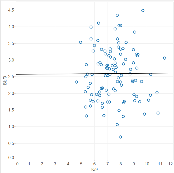
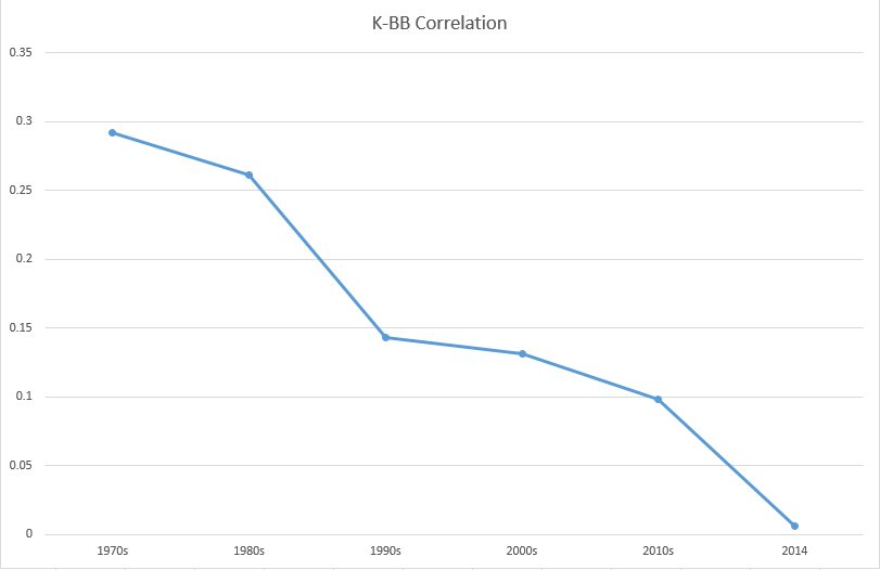
Although most studies of the “Curse” rarely delve into how players tweak their swings, it is likely safe to assume that they are changing their approach in the hope of belting as many homers as possible for that one night – developing an even greater power stroke. It is a commonly accepted conjecture that power and strikeouts are positively correlated (see Kendall 2014), meaning that greater power is associated with more strikeouts. This conjecture may not be as true for exceptionally talented players (i.e. Hank Aaron, Ted Williams, Mickey Mantle, Willie Mays, etc.) However, if we accept this assumption to be correct for the majority of players, it can be stated that if players change their swing to hit more home runs, they should see a corresponding increase in strikeouts in the second half of the season.[i] Thus, it can be hypothesized:

H2.1: Players who participate in the Home Run Derby will experience greater strikeouts per plate appearance in the second half of the season than those who did not participate in the Derby.

As with hypotheses 1.1 and 1.2, it can also be assumed that the effect of participation in the Derby will be greater the more swings an individual takes during the Derby. That is to say, if a player hits more home runs during the Derby, the altered swing he uses during the Derby will be more likely to carry through to the second half of the season. This leads to the hypothesis:

H2.2: Derby participants who hit more home runs in the Derby will experience greater strikeouts per plate appearance in the second half of the season than those who hit fewer home runs in the Derby (including those who do not participate).

In the next section of this study I will discuss the analytical approach, variable operationalization, and the data sources used to address the above four hypothesis.

Data and Analytical Method

Below I will begin with a discussion of the data used in this study. I will then discuss the independent and dependent variables for each hypothesis as well as the control variables used in this study. Finally, I will discuss the methodological approach used in this study.

Data Sources and Structure

Above, it is hypothesized that those players who either participated in the Derby, or performed well in the Derby will see greater offensive decline between season halves than those who either did not participate in the Derby, or struggled in the Derby. In order to properly test these hypotheses one must use data that includes those who participated in the Home Run Derby, and those who did not participate in the Derby.

This paper performs a meta-analysis of all players with at least 100 plate appearances in both the first and second halves of the season from 1985 (the first year in which the Home Run Derby was held) through 2013. This makes the unit of analysis of this paper the player-year. This data excludes observations from 1988 as the Derby was cancelled due to rain. Further, 1994 is also excluded as the second half of the season was cut short due to the players’ strike.

Independent Variables

The main independent variable for hypotheses 1.1, and 2.1 is a dichotomous measure of participation in the Home Run Derby. A player was coded as a 1 if they participated in the Derby and a 0 if they did not participate in the Derby. Between 1985 and 2013 a total of 229 player-years were coded as participating in the Derby.

The independent variable for hypotheses 1.2, and 2.2 is a measure of each player’s success in the Home Run Derby. This is an additive variable denoting the number of home runs each player hit in each year in the Derby. This variable ranges from 0 to 41 (Bobby Abreu in 2005). Those who did not participate in the Derby were coded as 0.[ii]

Dependent Variables

Hypotheses 1.1 and 1.2 posit that participation in the Derby and greater success in the Derby will lead to decreased power numbers respectively. Power hitting can be measured in numerous ways, the most obvious being home runs per plate appearance (HRPA). However, theoretically, if players are being sapped of energy, this should affect all power numbers, not simply HRPA. Restricting one’s understanding of power to HRPA ignores other forms of power hitting, such as doubles and triples. So as not to remove data variance unnecessarily, one can measure change in power hitting by using the difference between first and second half extra base hits per plate appearance (XBPA) rather than HRPA.

Thus, the dependent variable for hypotheses 1.1 and 1.2 is understood as the difference between XBPA in the first and second halves of the season for each player-year. XBPA is calculated by dividing the number of extra base hits (doubles, triples, and home runs) a player has hit by the number of plate appearances, thus providing a standardized measure of extra base hits for each player-year.

The dependent variable for hypotheses 1.1 and 1.2 was created by calculating the XBPA for the first half of the season, and the second half of the season for each player-year. The XBPA for the second half of the season for each player-year was then subtracted from the XBPA for the first half of the season for each player-year. Theoretically, this variable can from -1.000 to 1.000. In reality this variable ranges from -.116308 to .1098476, with a mean of -.0012872, and a standard deviation of .025814.

The dependent variable for hypotheses 2.1 and 2.2 is the difference between first and second half strikeouts per plate appearance (SOPA) for each player-year. SOPA is calculated by dividing the number of strikeouts a player has by his plate appearances, thus providing a standardized measure of strikeouts for each player-year.

The dependent variable for these hypotheses was created by calculating the SOPA for the first half of the season, as well as the second half of the season for each player-year. The SOPA for the second half of the season for each player-year was then subtracted from the SOPA for the first half of the season for each player-year. Theoretically, this variable can from -1.000 to 1.000. In reality this variable ranges from -.1857143 to .1580312, with a mean of -.003198, and a standard deviation of .0378807.

Control Variables

A number of control variables are included in this study. A dummy variable denoting whether a player was traded during the season is included.[iii] To control for the possible effects of injury in the second half of the season, a dummy variable denoting if a player had a low number of plate appearances in the second half of the season is included.[iv] Further, I include a dummy variable measuring whether a player had a particularly high number of first half plate appearances.[v] Finally, controls denoting observations in which the player played the entire season in the National League,[vi] observations that fall during the “Steroid Era,”[vii] observations that fall in a period in which “greenies” were tolerated,[viii] and observations that fall during the era of interleague play are included.[ix]

Analytical Approach

The main dependent variables used to test the above hypotheses are the difference between first and second half XBPA, and the difference between first and second half SOPA. For each of these variables, the data fits, almost perfectly, a normal curve.[x] For each of these variables, the theoretical range runs from 1 to -1, with an infinite number of possible values between. Although these variables cannot range from infinity to negative infinity, the most appropriate methodological approach for this study is OLS regression.

In the next section of this piece, I will report the findings of the tests of hypotheses 1.1 through 2.2. I will then discuss the implications of these findings.

Analysis

This section will begin with the presentation and the discussion of the findings concerning hypotheses 1.1 and 1.2. I will then present and discuss the findings of tests of hypothesis 2.1 and 2.2.

Analysis of Hypotheses 1.1 and 1.2

Column 1 of table 1 shows the results of the test of hypothesis 1.1. The intercept for this test is   -.0007, but is statistically insignificant. This suggests that, with all variables included in the test held at 0, players will see no change in their XBPA between the first and second halves of the season. The coefficient for the “Derby participation” variable shows a statistically significant coefficient of .008. This means, if a player participates in the Derby, he can expect to see his second half XBPA drop by .008.

Of course, there is a possibility that those who participate in the Derby will see a greater drop in their XBPA than the average player because, in order to be chosen for the Derby, a player will have a higher XBPA.[xi] This would then make it more likely that players who participate in the Derby see a greater drop in XBPA than players who do not participate as they regress to the mean. To account for this, the sample can be restricted to players with a high first half XBPA.

The mean first half XBPA for all players (those who do and do not participate in the Derby) between 1985 and 2013 is .0766589. The sample is restricted to only those players above this mean. This is done in for the tests displayed in column 2 of table 1. As can be seen, the intercept is statistically significant, with a coefficient of .01. Those who have average or above average XBPA in the first half of the season can expect to see their XBPA drop by .01 after the All-Star Break when all other variables in the model are held equal.

Table 1: The Effect of Home Run Derby Participation on the Difference in XBPA.

Note: Values above represent unstandardized coefficients, with standard errors in parentheses. *p<.05, **p<.01, ***p<.001

Turning to the Derby participation variable, one notices that it is now statistically insignificant with a coefficient of .02. When restricting the sample to only those who showed average or above average power in the first half of the season, the results show that those who participate in the Derby will see no statistically discernible difference in their power hitting when compared to those who did not participate in the Derby.

The variables denoting if a player had a low number of plate appearances in the second half of the season, or a high number of at-bats in the first half of the season, are statistically significant and both present with negative coefficients. Meaning if a player has a high number of at-bats in the first half of the season or if he has a low number of plate appearances in the second half of the season, he will actually see an increase in XBPA.

Although the results in column 2 of table 1 are telling, it may be useful to restrict the sample even further. Those who are selected for the Derby are, for all intents and purposes, the best power hitters in baseball. Therefore, one can restrict the sample to only the best power hitters and compare only those players with a first half XBPA equal to, or above the average for those who participated in the Derby, while, of course, keeping all Derby participants in the sample.

The mean first half XBPA for Derby participants between 1985 and 2013 is .1138781. Tests restricting the sample to only those with a first half XBPA of .1138781 are displayed in column 3 of table 1. The intercept for these tests is statistically significant and shows a coefficient of .04. Meaning those with a first half XBPA of .1138781 can expect to see a drop of .04 in their XBPA after the All-Star Break. The coefficient for the variable measuring participation in the Derby is -.004, but is statistically insignificant. This suggests that those who participate in the Derby do not see a marked decrease in their power hitting after the Derby when compared to those of similar power hitting prowess.

The only variable that shows a statistically significant effect in these tests is that which denotes whether a player had a high number of first half at-bats. As with previous tests, the coefficient for this variable is negative. This suggests that players who have a high number of first half at-bats see an increase in the XBPA between the first and second halves of the season in comparison to those without a high number of first half at-bats.

Columns 1 through 4 in table 2 show the tests of success in the Derby (the number of home runs hit) on the difference between first and second half XBPA. The test with a full sample is displayed in column 1 of table 2. The intercept for this test is statistically insignificant, suggesting that on average, players do not experience a marked change in their XBPA between the first and second halves of the season.

The variable denoting the number of home runs a player hit during the Derby is statistically significant and has a coefficient of .0003. This means that for every home run a participant in the Derby hit he can expect his XBPA after the All-Star Break to decline by .0003 points.

Of course, the relationship between Derby success and the difference in first half and second half XBPA is not likely to be linear, but rather curvilinear. Thus, a measure of home runs hit during the Derby squared should be included. The test including this variable is displayed in column 2 of table 2. The intercept is again statistically insignificant suggesting that when all variables in the model are held at 0, players should not see a marked change in their XBPA between the first and second half of the season.

Table 2: The Effect of the # of Home Runs Hit in the Derby on the Difference in XBPA.

Note: Values above represent unstandardized coefficients, with standard errors in parentheses. *p<.05, **p<.01, ***p<.001

The effect of success in the Derby remains statistically significant with a coefficient of .001. This means that with each home run a player hits in the Derby his XBPA in the second half of the season will decline by .001. Further, the variable “home runs squared” is statistically significant, and has a coefficient of -.00004. This indicates that the effect of the number of home runs a player hits in the Derby on second half production decreases with more home runs. In essence, hitting 40 home runs during the Derby does not have the same effect on second half offensive production as hitting 30 home runs during the Derby, and so on.

In terms of control variables, the variable denoting a high number of first half at-bats is statistically significant with a negative coefficient in the tests reported in column 1 of table 2. Further, in the tests reported in column 2 the variable denoting a diminished number of plate appearances in the second half of the season is statistically significant and negative.

As with the tests reported in table 1, restricting the sample to only those players with average and above average first half XBPA may be useful. Column 3 of table 2 shows the results of the test of the effect of success in the Derby on the difference in XBPA between the two halves of the season when the sample is restricted to those with a first half XBPA at or above the leagues’ average (.0766589).

The intercept in this test is statistically significant with a coefficient of .012. This means that, when all variables included in this test are held at 0, players with an average or above average first half XBPA notice a decline in the second half XBPA. Importantly, the effect of the number of home runs hit during the Derby is statistically insignificant, meaning that hitting more home runs during the Derby has no statistical effect on the difference between first half and second half XBPA when the sample is restricted to those with average or above average first half XBPA.

Both the variable denoting whether a player had diminished second half plate appearances, and the variable denoting whether a player had a high number of first half at-bats, are statistically significant with negative coefficients. This implies that those who experience a diminished number of second half plate appearances, and those players with a high number of first half at-bats see an increase in their XBPA between the first and second halves of the season.

Column 4 of table 2 restricts the sample based on the mean first half XBPA of those who participated in the Derby. The mean first half XBPA of these players is .1138781. The intercept for this test is statistically significant with a coefficient of .036. The variable measuring success in the Derby is statistically insignificant, meaning that the number of home runs a player hits in the Derby has no statistical effect on the difference between first and second half XBPA when comparing Derby participants to similar power hitters who did not participate in the Derby.

In terms of controls, the variable denoting whether a player had a high number of first half at-bats is again statistically significant with a negative coefficient. This, as with previous tests, suggests that those who have a high number of first half at-bats will experience an increase in XBPA between the first and second halves of the season.

Analysis of Hypotheses 2.1 and 2.2

The results of the tests of hypothesis 2.1 (participation in the Derby will lead to more strikeouts per plate appearance) are displayed in column 1 of table 3. This column shows the relationship between participation in the Derby and the change in SOPA between the first and second halves of the season. As can be seen, the intercept is -.006 and is statistically significant, meaning, all other things equal, players strikeout more often in the second half of the season.

The coefficient for “Derby participation” is -.005 and is statistically significant, meaning that those who participate in the Home Run Derby will see their second half SOPA increase by .005 between halves of the season in comparison to players who do not participate in the Derby. When one takes into account that SOPA should increase by .006 when all other variables are held at 0, this finding suggests that Derby participants should see an increase of .011 in their SOPA between the first and second halves of the season.

Unlike XBPA, there is very little chance that SOPA is associated with selection for the Home Run Derby. Moreover, the average first half SOPA for the entire sample used in this study is .1610312, whereas the mean first half SOPA for those who participated in the Home Run Derby is .1669383. Those who participated in the Derby were actually more likely to strikeout in any given plate appearance than those who did not participate in the Derby. Essentially, assuming that one should see a regression to the mean, it is more likely that those who participate in the Derby would see a decrease in SOPA between the first and second halves of the season. These results, however, tell the opposite story, and cannot be explained by a mere statistical anomaly. Therefore, it is unnecessary to restrict the sample, and one can state that hypothesis 2.1 is supported.

Turning to column 2 of table 3, one sees a test of hypothesis 2.2 (the more home runs a player hits in the Derby the smaller the difference between his first and second half SOPA will be). Much like the results in column 1 of table 3, the intercept is -.006 and is statistically significant. Thus, when holding all other variables at 0, one can expect the difference between a player’s first and second half SOPA to increase by .006.

The coefficient for the variable denoting the total number of home runs a player hit during the Derby shows a statistically significant coefficient of -.0005. For every home run a player hit during the Derby, the difference between his first half SOPA and second half SOPA will decrease by .0005.

This relationship, however, is likely curvilinear. In order to account for this likelihood I include a variable in which the total number of home runs a player hit during the Derby is squared. Column 3 of table 3 reports the results of a test including a measure of the total number of home runs squared. When this variable is included the coefficient of the total number of home runs becomes statistically insignificant. This suggests that the total number of home runs a player hit during the Derby is not related to the difference in that player’s first half SOPA and second half SOPA. It must be noted, however, that this finding does not negate the result in column 1 of table 3.

Interestingly, there are a number of control variables that show statistical significance in all tests included in table 3. If a player was traded midseason, he can expect to see the difference between his first half SOPA and second half SOPA to shrink, meaning he will see an increase in SOPA in the second half of the season. Further, having a below average number of plate appearances in the second half of the season leads to a decrease in second half SOPA.
class=Section9>

Table 3: The Effect of Home Run Derby Participation and the # of Home Runs Hit in the Derby on the Difference in SOPA.

Note: Values above represent unstandardized coefficients, with standard errors in parentheses. *p<.05, **p<.01, ***p<.001

The next section of this paper will first place the main findings of this paper in a broader context of the “Home Run Derby Curse.” It will then discuss possible avenues for further research.

Implications

The results above were mixed. In some instances, participation in the Derby, or success in the Derby, was statistically related to second half offensive decline, whereas in other tests, there was no relation between participation in the Home Run Derby and changes in offensive production between season halves. When using the full sample (N=7,330), the results showed that Derby participants can expect to see a greater drop in their XBPA between halves of the season than those who did not participate in the Derby. Moreover, those who have greater success in the Derby will see a greater drop in their XBPA between the first and second halves of the season in comparison to those who have not had as much success in the Derby. Further, the results showed, when using the full sample of players, those who participated in the Derby, as well as those who had greater success in the Derby, will, on average, expect to see their second half SOPA increase more than Derby non-participants.

These findings, however, must be discussed in closer detail. As McCollum and Jaiclin (2010) pointed out in their piece, some of these results may be due to the often extraordinary performances of Derby participants in the first half of the season, and any decline is simply a regression to the mean.

In order to address this issue, in testing the effect of Derby participation and success on change in XBPA, I restricted the sample to those who showed above-average and extraordinary performances in the first half of the season. The effect of Derby participation and success on change in XBPA disappeared when the sample was restricted to those who showed average or above-average first halves. This suggests that hypotheses 1.1 and 1.2 are not confirmed, and lends support to McCollum and Jaiclin’s regression to the mean conjecture.

Turning towards the relationship between Derby success and change in SOPA between halves, an effect was initially found. This suggests that those who hit more home runs during the Derby tend to see an increase in their second half SOPA in comparison to their first half SOPA. This relationship, however, evaporates when a measure of home runs squared in included. This suggests a lack of robustness to this finding, and thus hypothesis 2.2 cannot be confirmed.

Based upon these findings, it appears that the “Home Run Derby Curse” is more of a Home Run Derby myth. The results concerning Derby participation and SOPA, however, appear to tell a different story. The test of hypothesis 2.1 shows that those who participate in the Derby see a larger increase in their SOPA between halves of the season compared to players who do not participate in the Derby. As stated above, it is unnecessary to restrict the sample based upon first half SOPA because those who participate in the Derby have, on average, a higher first half SOPA than the full sample mean. Thus, the argument that Derby participants have had an exceptionally strong first half does not apply in the case of SOPA.

Simply put, derby participants do see a statistical increase in their SOPA in comparison to non-participants, suggesting that there is some credence to the “Home Run Derby Curse,” and, it is caused by players changing their swings. The question that remains, however, is what is the substantive impact of participation in the Derby on SOPA?

The Substantive Effect of Derby Participation on SOPA

Essentially, Derby participants can expect to see their second half SOPA increase by .005 more points over their first half SOPA than those players who do not participate in the Derby. The average first half SOPA for those who did not participate in the Derby is .1608855. The mean number of first half plate appearances for the sample used in this study, excluding those who participated in the Derby, is 249.5692. This means that the average Derby non-participant will strikeout about 41 times in the first half of the season.

With all variables in the model held equal, the average second half SOPA will be .006 points higher than the average first half SOPA, about .1668855. The mean number of second half plate appearances for the sample used in this study, excluding those who participated in the Home Run Derby, is 219.5873. Therefore, an average Derby non-participant will strikeout about 37 times in the second half of the season. When the first half and second half are combined, an average player who did not participate in the Home Run Derby can expect to strikeout about 78 times.

The mean first half SOPA for a Derby participant is .1669383. The average number of first half plate appearances for Derby participants is 356.9345. Thus, the average Derby participant can expect to strikeout about 60 times in the first half of the season.

The mean second half SOPA for a Derby participant can be understood as:

2^nd Half SOPA = .1669383+(-α)+(-β)

Where α is the intercept (-.006) and β (-.005) is the coefficient for participation in the Derby. All other variables held constant at 0, Derby participants can expect a second half SOPA of .1779383. The average number of second half plate appearances for Derby participants is 291.7209. With all variables other than “Derby participation” held equal at 0, those who participate in the Derby can expect about 52 strikeouts in the second half of the season. This suggests that a Derby participant can expect to strike out 112 times during the season.

This is a substantial difference in strikeouts, however, in order to accurately assess the true substantive effect of Derby participation, one must utilize a common number of plate appearances across both Derby participants and non-participants alike. For the purposes of this paper, I make the reasonable assumption that players will have about 300 plate appearances in the second half of the season.

Using 300 plate appearances, those who did not participate in the Derby can expect 50 strikeouts in the second half of the season, whereas those who did participate in the Derby can expect 53 strikeouts in the second half of the season.[xiv] This difference of three strikeouts does not seem substantively large.

Further, it must be noted that the coefficient for Derby participation of -.005 is only an estimate with a 95% confidence interval ranging from -.0002 to -.01. If the true coefficient is -.01, this would amount to about 5 more strikeouts over 300 plate appearances in the second half of the season. If the true coefficient is -.0002, a player who participates in the Derby could expect, all other things held equal, to strikeout 2 more times over 300 plate appearances in the second half of the season than a player who did not participate. In essence, the difference in SOPA between the halves of the season due to participation in the Derby is statistically significant, but substantively negligible.

Broader Implications and Future Research

Although the effects of Derby participation on SOPA are substantively minimal, the take away point of this study is that a “Home Run Derby Curse” does exist. Further, the confirmation of H2.1 suggests that Derby participants are altering their swings to develop more power during the Derby, and this is affecting their swing in the second half of the season.

Regardless of the substantive effects, this is an important finding. If a Derby participant’s swing is altered so greatly that they begin striking out at an even faster rate than non-participants in the second half of the season, the question that we must ask is, what other effects does this altered swing have? Does it increase a Derby participant’s flyball ratio? Are Derby participants more likely to see a drop in batting average and walks?

Beyond these questions, future research into the “Curse” should also focus on how the Derby alters a player’s swing. One possible avenue for future research lies in measuring changes in a hitter’s stance (i.e. distance between their feet, angle of their back elbow, etc.) after the Derby relative to a player’s stance prior to the Derby.

Works Cited:

 J.P. Breen, “The Home Run Derby Curse,” FanGraphs, July 11, 2012, accessible via http://www.fangraphs.com/blogs/the-home-run-derby-curse/.

Jason Catania, “Is there Really a 2^nd-Half MLB Home Run Derby Curse?,” Bleacher Report, July 15, 2013, accessible via http://bleacherreport.com/articles/1702620-is-there-really-a-second-half-mlb-home-run-derby-curse.

Derek Carty, “Do Hitters Decline After the Home Run Derby?,” Hardball Times, July 13, 2009, accessible via http://www.hardballtimes.com/do-hitters-decline-after-the-home-run-derby/.

Evan Kendall, “Does more power really mean more strikeouts?,” Beyond the Box Score, January 12, 2014, accessible via http://www.beyondtheboxscore.com/2014/1/12/5299086/home-run-strikeout-rate-correlation.

Tim Marchman, “Exploring the impact of the Home Run Derby on its participants,” Sports Illustrated, July 12, 2010, accessible via http://sportsillustrated.cnn.com/2010/writers/tim_marchman/07/12/hr.derby/.

Joseph McCollum, and Marcus Jaiclin. 2010. “Home Run Derby Curse: Fact or Fiction?,” Baseball Research Journal 39(2).

[i] It could be argued that those players who participate in the Derby are also exceptional players, and therefore, this conjecture will not be correct for the majority of those who participate in the Derby. At first glance, this would appear to create a problem for the analysis in this piece, however, this is not so. This would only present a problem if being exceptional led to a greater positive correlation between a power swing and strikeouts, that is if a power stroke for exceptional players leads to more strikeouts than a power stroke for average players. If exceptional hitters are less likely to have a positive correlation between power and strikeouts, and Derby participants are exceptional players, we would expect to see a lower strikeout rate among these players when they begin attempting to hit for greater power. Essentially, a violation of this assumption leads to a more conservative measurement.

[ii] Some players who participated in the Derby were coded as “0,” as they did not hit any home runs.

[iii] A player is coded as a 1 if he was traded during the season and a 0 if he was not traded.

[iv] A player is coded as a 1 if the difference in his plate appearances between the first and second halves of the season (Pre All-Star Break PAs – Post All-Star Break PAs) is greater than the observed average in the data (39.8). A player is coded as a 0 if the difference in his plate appearances between the first and second halves of the season is less than the observed average in the data.

[v] A player is coded as a 1 if the number of plate appearances he had during the first half of the season is greater than the observed average in the data (342).

[vi] This variable is a dummy variable, with a player being coded as a 1 if he spent the entire season in the National League, and a 0 if he did not spend the entire season in the National League.

[vii] Although the “Steroid Era” is somewhat difficult to nail down, for the purposes of this paper, it is assumed to run from 1990 through 2005. Therefore, if an observation is in or between 1990 and 2005 it is coded as a 1. If an observation falls outside of this time period it is coded as a 0.

[viii] For the purposes of this paper, the era of “greenies” is deemed to run from 1985 through 2005. Therefore, if an observation is in or between 1985 and 2005 it is coded as a 1. If an observation falls outside of this time period it is coded as a 0.

[ix] Interleague play began in 1995 and continues through present. Therefore, if an observation is in or between 1995 and 2013 it is coded as a 1. If an observation falls outside of this time period it is coded as a 0.

[x] The difference in XBPA variable maintains the same basic distribution when the sample is restricted to those with an XBPA equal to or greater than the league average (.0766589), as well as equal to or greater than the Derby participant average (.1138781).

[xi] The mean first half XBPA for those who participate in the Derby is .114, whereas the mean first half XBPA for those who do not participate in the Derby is .077.

[xii] When this model is run including a variable for “home runs squared” the results remain similar.

[xiii] When this model is run including a variable for “home runs squared” the results remain similar.

[xiv] One could quibble with the estimate of 300 second half plate appearances, however, it is important to note that a Derby participant’s second half strikeout total increases over a non-participants strikeout total by .5 for every 100 plate appearances. Thus, if one were to use 200 plate appearances, the difference in average strikeout totals between Derby participants and non-participants for the second half of the season would be about 2.5. Additionally, if one were to use 400 plate appearances, the difference in average strikeout totals between Derby participants and non-participants for the second half of the season would be about 3.5.

I think the National League West is the most idiosyncratic division in baseball. Note that I avoided a more disparaging term, like odd or weird. That’s not what I’m trying to convey. It’s not wrong; it’s just…off. Not bad–it’s home to 60% of the last five World Champions, right?–but different. Let me count the ways. (I get three.)

Time zones

EAST COAST BIAS ALERT!

It is difficult for people in the Eastern time zone to keep track of the NL West. Granted, that’s not the division’s fault. But 47% of the US population lives in the Eastern time zone. Add the Central, and you’re up to about 80%. That means that NL West weeknight games generally begin around the time we start getting ready for bed, and their weekend afternoon games begin around the time we’re starting to get dinner ready. The Dodgers, Giants, and Padres come by it naturally–they’re in the Pacific time zone. The Diamondbacks and Rockies are in the Mountain zone, but Arizona is a conscientious objector to daylight savings time, presumably to avoid prolonging days when you can burn your feet by walking barefoot outdoors. So effectively, four teams are three hours behind the east coast and the other team, the Rockies, is two hours behind.

Here’s a list of the number of games, by team, in 2015 that will be played in each time zone, ranked by the number of games in the Mountain and Pacific zones, counting Arizona among the latter:

Again, I’m fully on board with the idea that this is a feature, not a bug. But it’s a feature that means that a majority, or at least a solid plurality, of the country won’t know, for the most part, what’s going on in with the National League West teams until they get up in the morning.

Ballparks

OK, everybody knows that the ball flies in Coors Field, transforming Jose Altuve to Hack Wilson. (Check it out–they’re both 5’6″.) And the vast outfield at Petco Park turns hits into outs, which is why you can pencil in James Shields to lead the majors in ERA this year. But the other ballparks are extreme as well: Chase Field is a hitter’s park; Dodger Stadium and AT&T Park are pitchers’ havens. The Bill James Handbook lists three-year park factors for a variety of outcomes. I calculated the standard deviations for several of these measures (all scaled with 100 equal to league average) for the ballparks in each division. The larger the standard deviation, the more the ballparks in the division play as extreme, in one direction or the other. The NL West’s standard deviations are uniformly among the largest. Here’s the list, with NL West in bold:

• Batting average: NL West 10.1, AL West 7.2, AL Central 6.5, AL East 5.8, NL East 5.2, NL Central 1.6
• Runs: NL West 26.5, NL Central 7.9, NL East 6.9, AL East 4.0, AL Central 2.8, AL West 2.7
• Doubles: AL East 20.3, NL West 11.3, NL East 6.2, NL Central 5.9, AL Central 5.1, AL West 2.9
• Triples: NL West 50.6, AL Central 49.5, NL East 33.6, AL West 28.3, AL East 27.8, NL Central 11.1
• Home runs: NL Central 30.2, NL West 23.9, NL East 20.0, AL East 18.7, AL Central 11.3, AL West 11.2
• Home runs – LHB: NL Central 31.6, AL East 27.4, NL West 25.6, NL East 21.7, AL West 14.7, AL Central 11.7
• Home runs – RHB: NL Central 32.1, NL West 24.0, NL East 20.0, AL East 14.4, AL Central 13.6, AL West 10.2
• Errors: AL East 17.7, NL West 12.2, NL Central 11.6, NL East 11.5, AL West 11.2, AL Central 8.2
• Foul outs: AL West 36.2, AL East 18.3, NL West 16.0, NL Central 15.2, AL Central 13.8, NL East 6.2

No division in baseball features the extremes of the National League West. They ballparks are five fine places to watch a game, but their layouts and geography do make the division idiosyncratic.

Social Investing

You may be familiar with the concept of social investing. The idea is that when investing in stocks, one should choose companies that meet certain social criteria. Social investing is generally associated with left-of-center causes, but that’s not really accurate. There are liberal social investing funds that avoid firearms, tobacco, and fossil fuel producers and favor companies that offer workers various benefits. But there are also conservative social investing funds that don’t invest in companies involved in alcohol, gambling, pornography, and abortifacients. This isn’t a fringe investing theme: By one estimate, social investing in the US totaled $6.57 trillion at the beginning of 2014, a sum even larger than the payrolls of the Dodgers and Yankees combined.

Here’s the thing about social investing: You’re giving up returns in order to put your money where your conscience is. That’s OK, of course. The entire investing process, if you think about it, is sort of fraught. You’re taking your money and essentially betting on the future performance of a company about which you know very little. Trust me, I spent a career as a financial analyst: I don’t care how many meals you eat at Chipotle, or how many people you know at the Apple Genius Bar, you can’t possibly know as much about the company as a fund analyst who’s on a first-name basis with the CEO. So there’s no sense in making it even harder on yourself by, say, investing in the company guilty of gross negligence and willful misconduct in a major oil spill, if that’d bother you.

Note that I said that with social investing, you’re giving up returns. Some social investing proponents would disagree with me. They claim that by following certain principles that will eventually sway public opinion or markets or regulations, they’re investing in companies that’ll perform better in the long run. That’s a nice thought, but social investing has been around for decades, and we haven’t yet hit that elusive long run. The Domini 400 Index, which was started in 1990, is the oldest social investing index. It started well in the 1990s, but has lagged market averages in the 21st century. Now called the MSCI KLD 400 Social Index, it’s been beaten by the broad market in 10 of the past 14 years. It’s underperfomed over the past year, the past three years, the past five years, and the past ten years, as well as year-to-date in 2015. The differences aren’t huge, but they’re consistent. Maybe for-profit medicine in an aberration, but acting on that meant that you missed the performance of biotechnology stocks last year, when they were up 47.6% compared to an 11.4% increase for the S&P 500. Maybe we need to move toward a carbon-free future, but stocks of energy companies have outperformed the broad market by over 100 percentage points since January 2000. I think that most social investing investors are on board with this tradeoff, but some of the industry proponents have drunk the Kool-Aid of beating the market. That’s just not going to happen consistently. In fact, a fund dedicated to tobacco, alcohol, gambling, and defense (aka “The Four B’s:” butts, booze, bets, and bombs) has outperformed the market as a whole over the past ten years.

OK, fine, but what does this have to do with the National League West? Well, two of its members have, in recent years, made a point of pursuing a certain type of player, just as social investing focuses on a certain type of company. The Diamondbacks, under general manager Kevin Towers and manager Kirk Gibson, became a punchline for grit and dirty uniforms and headhunting. (Not that it always worked all that well.) The Rockies, somewhat less noisily, have pursued players embodying specific values. Co-owner Charlie Monfort (a man not without issues) stated back in 2006,  “I don’t want to offend anyone, but I think character-wise we’re stronger than anyone in baseball. Christians, and what they’ve endured, are some of the strongest people in baseball.” Co-owner Dick Monfort described the team’s “culture of value.” This vision was implemented by co-GMs (hey, Colorado starts with co, right?) Dan O’Dowd and Bill Geivett. (OK, O’Dowd was officially GM and Geivett assistant GM, but the two were effectively co-GMs, with Geivett primarily responsible for the major league team and O’Dowd the farm system).

Now, there’s nothing wrong with players who are also commendable people. You could do a lot worse than start a team with Clayton Kershaw and Andrew McCutchen, to name two admirable stars. Barry Larkin was a character guy. So was Ernie Banks. Brooks Robinson. Walter Johnson. Lou Gehrig. All good guys.

But holding yourself to the standards set by the Diamondbacks and Rockies also means you’re necessarily excluding players who are, well, maybe more characters than character guys.  Miguel Cabrera has proven himself to be a tremendous talent and a somewhat flawed person. Jonathan Papelbon has a 2.67 ERA and the most saves in baseball over the past six years, but he’s done some things that are inadvisable. Carlos Gomez, a fine player, second in the NL in WAR to McCutchen over the past two years, has his detractors. Some of the players whom you’d probably rather not have your daughter date include Babe Ruth, Ty Cobb, Rogers Hornsby, Barry Bonds, and many of the players and coaches of the Bronx Zoo Yankees.

I want to make a distinction here between what the Diamondbacks and Rockies did and the various “ways” that teams have–the Orioles Way, the Cardinals Way, etc. There’s plenty of merit in developing a culture starting in the low minors that imbues the entire organization. That’s not what Arizona and Colorado did. They specified qualities for major leaguers, and, in the case of the Diamondbacks at least, got rid of players who didn’t meet them. I don’t know what’s wrong with Justin Upton, but for some reason, Towers didn’t like something about him, trading him away. The Braves make a big deal about character, but of course they traded for Upton, so the Diamondbacks went way beyond anything the Braves embrace.

In effect, what the Diamondbacks and Rockies have done is like social investing. They’ve viewed guys who don’t have dirty uniforms or aren’t good Christians or something the same way some investors view ExxonMobil or Anheuser-Busch InBev. Again, that’s their prerogative, but it loses sight of the goal. Investors want to maximize their returns, but as I said, most social investors realize that by focusing on only certain types of stocks, they’ll have slightly inferior performance. They’ll give up some performance in order to hew to their precepts. Baseball teams want to maximize wins, and there really isn’t any qualifier related to precepts you can append to that.

The Rockies and Diamondbacks were living under the belief that by focusing on only certain types of players, they could have superior performance. It’s like the people who think they can beat the market averages through social investing. It hasn’t happened yet. And, of course, the Diamondbacks and Rockies were terrible last year, with the worst and second-worst records in baseball. Just as social investing doesn’t maximize profits, the baseball version of social investing didn’t maximize wins in Phoenix or Denver.

I’ve used the past tense throughout this discussion. Towers, Gibson, O’Dowd, and Geivett are gone, replaced by GM Dave Stewart and manager Chip Hale in Arizona and GM Jeff Bridich in Colorado. (The Monforts remain.) Last year, the Diamondbacks created the office of Chief Baseball Officer, naming Tony LaRussa, a Hall of Fame manager who’s been less than perfect as a person and in the types of players he tolerates. These moves don’t change that these are both bad teams. But by pursuing a well-diversified portfolio of players going forward, rather than a pretty severe social investing approach, both clubs, presumably, can move toward generating market returns. Their fans, after all, never signed on to an approach that willingly sacrifices wins for the sake of management’s conscience.

Yesterday, Nate Andrews asked the following question on Carson’s Instagraphs post 

I’m jus a little curious of the idea of length to reach the major leagues though. It’s definitely interesting to see the difference between high school and college draftees, but I’d be interested in looking at say, the average length to reach the major leagues (especially in first round draftees, considering they make it more often). On average, does it take a high school kid significantly longer to compared to someone who went to a 4 year college? I’d assume yes, but just something I would find interesting to see.

To answer that question, I did a very quick analysis. I compiled all first-round draft picks including supplemental first-rounders from 2008-2011 (dates arbitrarily chosen). Of those 200 players, 87 of them have reached the majors. Ignoring the three JC players, we are left with the following average time to majors:

HS: 3.8 years
4 Year: 2.5 years

So from this it appears that it takes high-school players a little over a year longer than college players, at least for those taken in the first round.

Of course, this analysis has a huge flaw, namely that I’m ignoring those 113 players that haven’t reached the majors. Many of them never will, but several will get there, thus biasing my numbers too low.

To deal with issue, I turned to something in statistics known as survival analysis. The name stems from biostatistics, where as the name implies, they are interested in the time until an individual dies. However, many medical studies are only run for a few years, and inevitably some individuals do not die in the period. Thus the idea of ‘censoring’ was born, where we know that someone survived until some time, but we do not know when they will actually die. These individuals still provide information for the researchers, which is modeled using a censoring mechanism. If anyone is interested in survival analysis, there are tons of references, but you can start with Wikipedia.

However, in biostatistics, we typically know that the event will eventually occur. However, in our context (time to reach majors), an event may not occur. There are good ways to deal with this, but I am going to be lazy. Instead, I just dropped the four players from my group that have not played professionally since 2002. This will likely bias the numbers too high, but still provides a fun exercise.

Once we account for censoring, the average time to majors is now:

HS: 6.5 years
4 Year: 4.5 years

While biased high, the difference between high school and college should not be affected. Now we have evidence that it takes high-school players about two more years than college players, at least on average. For those interested, JC players come in at 4.7 years (extremely small sample size warning!).

Just for fun, I did a similar analysis for draft position and position. Again, these numbers will be biased a little too high, but are interesting nonetheless.

The first overall pick is expected to reach the majors in 3.6 years. For every pick after that, we expect an additional 0.07 years, on average, to reach the majors. Thus the 10th overall pick should reach the majors in ~4.3 years, the 30th overall in 5.7 years, and so forth.

For position, a player’s position is whichever position is assigned to him on Baseball Reference’s draft page. I have no idea if this represents their position on draft day, or something else. Left fielders and right fielders are lumped together here. The results are as follows:

C: 5.0 years
1B: 3.1 years
2B: 4.5 years
3B: 3.9 years
SS: 5.1 years
LF/RF: 6.3 years
CF: 5.6 years

RHP: 5.9 years
LHP: 5.5 years

It should be said again that these numbers are a bit high. Furthermore, I am well aware that the sample size is low, so expect rather high uncertainty on these numbers. If anyone wants to further this analysis, I highly encourage it!

If you want to email someone for any reason, please feel free to email this specific someone at SomeoneOnFangraphs@gmail.com.

Rob Arthur published a really interesting piece at Baseball Prospectus, where he presented evidence in favor of the idea that batters are aware of the relative framing ability of the receiver they’re facing. That’s really fascinating to me, because it suggests that this skill, which the baseball research community has only recently begun to quantify, has been understood by players for a long enough time to show up in the behavior of major leaguers.

If that were true, batters are not the first component of an at-bat I’d expect to adjust to the receiver. Quotes from pitchers in the past have suggested that they’re aware of when their catcher is helping them out, and how; I want to know if that awareness is reflected in their pitch tendencies. Specifically, I want to know if pitchers are aware of the particular framing skills of their receivers. This article, by Community Blog Overlord Jeff Sullivan, is a little old, but it was one of the first framing articles I read, and the first I remember suggesting that some catchers were not just better at framing than their counterparts, but framing in specific parts of the zone. This more recent article, where Dave Cameron discusses the possibility of voting for Jonathan Lucroy as NL MVP, does talk about pitcher tendencies based on receiver skill, but it’s one pitcher and one catcher. Additionally, I’m just as interested to see how pitchers react to bad receivers, which as far as I can tell, hasn’t been covered. Do pitchers throw to their receivers’ strengths, and do they avoid their weaknesses?

The first thing to do is to establish how catchers do in different sections of the strike zone. I’m using Pitch F/X data from the wonderful Baseball Savant, which splits the zone like so:

For the purposes of this article, I’m concerned with the relative ability of receivers to preserve and gain strikes in different parts of the zone. As such, I’m going to categorize all pitches as “high in-zone” (in zones 1, 2, and 3), “high out-zone” (11 and 12), “low in-zone” (zones 7, 8, and 9), and “low out-zone” (13 and 14). It is a little unfortunate that this doesn’t pick up the relative horizontal skill of receivers, but these divides should still allow for some real differentiation between catchers while also keeping our sample sizes large-ish. If we pick too narrow a slice of the zone, the results might get a bit iffy.

Calculating relative framing ability took a few steps. To begin with, I looked at receivers with at least 30 pitches in each of the four zones, which picks up 87 catchers. That’s might be way too small a sample size, but the least pitches caught by any of these receivers is 1,040, which is not terrible. For each receiver, I calculated their rate of strikes for each of the four zones, and took the ratio between their strike rate and the average strike rate for the sample, and averaged together that ratio for the two low zones and the two high zones. That left two ratios for each player, high and low, where a number greater than 100 indicated better than average framing ability and a number less than 100 indicated worse than average framing ability.

Now, this is not a very good framing metric, but it does allow for a zone-oriented measure. I then divided the high-zone ratio by the low-zone ratio to get a final ratio, where greater than 100 indicated a receiver relatively better at getting the high strike, and less than 100 indicated a receiver relatively better at getting the low strike. Catchers notably better in the lower part of the zone: George Kottaras (.68), Jeff Mathis (.72), and Travis d’Arnaud (.73). Jonathan Lucroy, mentioned as a good low-ball framer, had a score of .89, but as he was good in both parts of the zone, there was a limit to how extreme his ratio could be. Catchers notably better in the high part of the zone: A.J. Ellis (1.46), Adrian Nieto (1.33), and Brett Hayes (1.29), again, three catchers with pretty bad receiving reputations.

So we now have a rough indication of how much better catchers are in the bottom and top of the zone. What kind of relation does this have to how they were pitched to? To estimate that, I stayed simple – I ran a linear regression, with the high/low ratio as the independent variable and the percentage of low or high pitches the catcher was thrown as the dependent variable. This, again, is a very rough measurement, since different pitchers are throwing to these catchers, but looking on a battery-by-battery basis would make the sample sizes tiny. Additionally, sometimes a catcher is catching a given pitcher because he’s good at receiving in a certain part of the zone that pitcher throws to frequently. So while this might be picking up manager actions as well as pitcher actions, it should be picking up something.

Results! Two graphs.

Both graphs show the expected relationship, with this blunt measurement of relative framing ability doing a fairly good job of predicting the distribution of low and high pitches thrown to a given catcher. Obviously there’s more at play here, but clearly pitch selection is impacted by the strengths of the receiver behind the plate.

There’s another question that can potentially be answered using this metric: do pitchers react differently to strengths and weaknesses? If one catcher is 30% better at framing low pitches than high pitches, and very good at framing low pitches, and another catcher is also 30% better at framing low pitches than high pitches, but very bad at it (and apparently even worse at framing high pitches, I guess (he is a very good hitter)), is one of them more likely than the other to get an increased rate of low pitches? In other words, are pitchers more inclined to avoid the bad, or seek the good?

To answer this question, I split the receivers into above-average and below-average low pitch receivers (46 and 41 in each group) and above-average and below-average high pitch receivers (51 and 36 in each group), using the scale described above. I then plotted the rate of pitches in the appropriate zone against each group separately. Following: more graphs!

What we see here is a higher R² value in both of the below-average samples, indicating that the high vs. low ability of bad framers appears to influence pitcher decisions more than the high vs. low ability of good framers. The gap for low pitches isn’t huge, but the gap for high pitches is fairly substantial. While this analysis is way too rough to conclusively show anything, this would seem to suggest that pitchers behave differently when throwing to good and bad framers, and may be more inclined to avoid weaknesses than to seek out strengths.

As I said (several times), this is a rough analysis that relies on a rough metric, but I think it provides some evidence for some very interesting pitcher behavior. I’d love to hear about other ways of identifying receivers’ strengths and weaknesses in different parts of the zone, so if anyone knows of articles doing so, or has some different ideas, say so in the comments!

Hello World! As a software developer, automation is my way of life. It kills me to see the tedious yet important job of calling balls and strikes performed at less than 90% accuracy. Worse, catcher framing is now a thing, which is essentially baseball’s equivalent of selling the flop.

Today, I want to talk about how automating the strike zone would affect the MLB run-scoring environment. Don’t we all want to save the environment?

Let’s pretend that before the 2014 season, home plate umpires were fitted with earpieces giving them a simplified Pitch f(x) feed of balls and strikes. They heard a high beep for a strike, a low beep for a ball. They then called balls/strikes exactly as they were told, resulting in a perfect zone.

Experiment 1: Walks/Strikeouts overturned

The most damaging ball/strike errors happen when ball 4 or strike 3 was thrown but not called. Sometimes the umpire is redeemed by luck, and a walk/strikeout happens eventually anyway, but not nearly every time. Think of how many times you’ve seen a 3–0 count where a ball was called a strike, only to have the hitter swing and ground out harmlessly on the 3–1 pitch.

For these experiments, let’s look at short description of the situation, the number of instances of that situation in 2014, and net runs that would have been added if a perfect zone had been called.

Data courtesy of Baseball Savant; click on a situation to see the query I used.

Are you surprised? The umpires made 545 more extra outs than extra ‘safes’. Using a rough walk minus out run differential of 0.6 runs, we see that a perfect zone would have added 0.07 runs per game. Interesting, but not huge.

But think again—this effect isn’t limited to plate appearances that should have ended with a bad call. We all know that the count affects the expected run value all on its own. So let’s expand this to all ‘bad calls’ in 2014.

Experiment 2: All balls/strikes called correctly

Balls and strikes don’t obviously translate to runs. So I’ll use someone else’s much more careful research and use a ball minus strike run value of approximately 0.14 runs. Here’s what happens when we apply a perfect zone to all balls and strikes. Brace yourself!

Whoa. Are you kidding me? If we’d run last season with a perfect strike zone, the run environment would go from 4.07 runs/game to nearly 5! That’s the highest level since 2000. I know what you’re thinking: this is crazy, and probably wrong.

Sanity checking

I also found this result to be larger than expected, to say the least. So let’s back up, check the mirrors, and look at the frequency of called strikes vs. balls.

There are a ton more called balls than called strikes. This makes sense because batters are more likely to swing at strikes. But the ratio of balls to strikes is only about 2:1, that doesn’t account for the 5:1 ratio among ‘mistaken’ balls/strikes! How do we account for this?

A possible explanation

Here we dive into speculation, but stay with me for a minute. Maybe there’s a logical explanation.

What sequence of events must occur in order for a Pitch f(x) strike to become a ball?

1. Pitcher throws in strike zone: ~45% (Zone %)
2. Hitter takes said pitch in the strike zone: ~35% (100% – Z-Swing %)
3. Umpire makes bad ‘ball’ call: ~10%

By this ridiculously rough method, we would expect bad ‘ball’ calls about 1.5% of the time (0.10 * 0.35 * 0.45). Compare that with the observed value of 1.2%

Conversely, the sequence for a Pitch f(x) ball becoming a called strike is as follows:

1. Pitcher throws out of zone: ~55% (100% – Zone %)
2. Hitter takes said pitch outside the strike zone: 70% (100% – O-Swing %)
3. Umpire makes bad ‘strike’ call ~15%

We therefore expect bad ‘strike’ calls about 5.7% of the time (0.15 * 0.7 * 0.55). Again, compare that to the observed value of, wait for it, 5.7%. Boom!

More reasons to automate

1. Automatic things happen faster. As a professional automator, I guarantee this will speed up play, by more than you think. I bet the umpire thinks for about 1 second on every pitch. That’s just the obvious part.
2. Set the umpires free. Focusing on something as difficult as calling balls/strikes squeezes out the umpire’s attention on other important matters, such as enforcing pace of play.
3. Crazy cool things will happen. For example, we will finally see what happens to an insane control pitcher’s K-BB%. V-Mart might never strike out!

I welcome your comments, criticisms, or even praise 🙂

For every Dontrelle Willis–who continues to get looks from Major League teams despite over eight years of complete ineptitude–there exists a handful of other players who fade into relative obscurity only a year or two removed from a dominant season. All it generally takes is a down year resulting from–or paired with–an injury to send a guy spiraling below the radar. These are often the players that can return the most value during fantasy drafts if you can make the distinction between a year that’s an aberration, and one that is a bellwether for a significant, irreversible decline in skills.

While I can’t say with complete confidence that Curtis Granderson’s 2014 doesn’t fall into the latter category, there were a couple of encouraging things going on below the subpar surface stats that make me think he can return some solid value this year, especially considering where he’s going in most drafts.

Granderson was 33 last year and coming off an injury-shortened season. He was also trading a left-handed pull hitter’s haven in Yankee Stadium for the cavernous confines of Citi Field. All things considered, it was natural to expect some significant regression. And when he hit .136 through his first 100 at-bats of the season, it seemed like the Mets might have had a disaster of Jason Bay-like proportions on their hands.

Fortunately for them, Granderson managed to right the ship to an extent, putting together a couple of excellent months. His final line of .227/.326/.388–dragged further down by a nightmarish .037 ISO, 16-for-109 August–wasn’t spectacular by any stretch. But there were some nice takeaways buried in there.

For one, his bat speed doesn’t seem to have slowed enough to justify the statistical hits he took across the board. Despite seeing 56.3% fastballs–the most he’s seen since 2010 by a wide margin–his Z-Contact % of 85% was in line with his 85.8% career average, and not far removed from the league average of 87%. I suspect the uptick in fastballs resulted from opposing teams banking on an age-slowed swing, but Granderson’s contact rates on high velocity pitches in the zone didn’t suffer for it.

Granderson also set a career high in O-Contact % with a 62.7% rate. This could usually indicate a lack of plate discipline as much as it could a sustained bat speed, except that Granderson’s O-Swing % of 26.2% is roughly the average of what he did in the four years prior. He also managed to post the second-highest walk rate of his career (12.1%) and his lowest strikeout percentage since 2009 (21.6%). These are not particularly impressive rates in their own right, but in the context of Granderson’s career they do help to dispel the notion that last year was the beginning of the end for his hitting ability.

That is not to say, of course, that I foresee a return to the 40 home run, .260+ ISO form that he flashed in his early Yankee years–there’s no way he ever touches the absurd 22 HR/FB% that sustained that run. But with the right field fences at Citi Field moving in–a change that apparently would have resulted in 9 more home runs for Granderson had it been done last season–and some improvement on last year’s uncharacteristically bad .265 BABIP, I would not be at all surprised to see a home run total between 25 and 30 to go along with double-digit steals and a batting average that won’t kill you. And that has value when it is being drafted as low as Granderson currently is.

As offense is continuously decreasing, a popular suggestion to increase the offense has been the shrinking of the strike zone. Primarily discouraging the low strike — since the implementation of QuesTec and later Zone Evaluation, the low strike is being called more and more often. All it really is is the enforcement of the strike zone or the rule of the strike zone. The solution that many have proposed is to reduce the low strike, which would require a changing in the wording of the strike zone. This in theory would increase the offense, which would increase the popularity of the game.

This may be a surprise to some but the re-wording of the strike zone is a common occurrence throughout the history of the game. Ok, maybe not common but it does happen on occasion. The first implementation of a strike zone was in 1887. Before 1887 batters would ask where they wanted the ball delivered and pitchers had to throw it there. There was no official definition of the strike zone.

The main question I tried to answer was how did the re-wording of the strike zone affect the run environment, if at all? There is no guarantee that it has, or that there is a correlation between the change in strike zone rules and the run environment. I think it’s a good theory and I would tend to believe that it would affect the run environment; that being said there are many factors that go into the run environment, and the strike zone is merely one of them.

The first chart is a representation of the run environment leading up to 1887, when the strike zone was officially defined. The definitions of the strike zone were found on Baseball Almanac. The data for all the charts was provided by baseball-reference. The X-axis for all the upcoming charts is the year and the Y-axis is the average runs per game.

Take this data for what you will. I personally don’t think it truly reveals a ton about the strike zone’s effect but it is a data point.

“A (strike) is defined as a pitch that ‘passes over home plate not lower than the batsman’s knee, nor higher than his shoulders.”

After 1887 there was a relatively steep drop in the run environment before it went back up. I’m not entirely sure the data reveals anything; the chart is rather noisy. In this chart, probably other factors were conducive to the fluctuation in run environment.

“A fairly delivered ball is a ball pitched or thrown to the bat by the pitcher while standing in his position and facing the batsman that passes over any portion of the home base, before touching the ground, not lower than the batsman’s knee, nor higher than his shoulder. For every such fairly delivered ball, the umpire shall call one strike.”

This chart again isn’t precisely indicative that the change in strike zone had an impact on the run environment. The modern game was still in its infancy and there was a lot of fluctuation before things stabilized in the mid 1900s.

“The Strike Zone is that space over home plate which is between the batter’s armpits and the top of his knees when he assumes his natural stance”.

This data point gives us more information. There was a pretty drastic drop from 1950-1952 in offense. In fact it was almost an entire run of offense that dropped and it makes sense. This was the first time there was a concrete definition of the strike zone. The umpires now had something to go on. Before there was a general idea of what strike and ball was. This was the first acknowledgment that there was a concrete zone pitchers had to throw into. The run environment did stabilize though until1963, where there was a slight drop in offense, obviously unrelated to the strike zone.

“The Strike Zone is that space over home plate which is between the top of the batter’s shoulders and his knees when he assumes his natural stance. The umpire shall determine the Strike Zone according to the batter’s usual stance when he swings at a pitch.” This rule was implemented in 1963.

As you can see there is no real change or effect from the rule change or the re-working of the rule. What you will also be able to conclude from the upcoming charts is that the re-wording of the strike zone doesn’t exactly have any effect on the offensive environment.

The strike zone was then again altered in 1969; “The Strike Zone is that space over home plate which is between the batter’s armpits and the top of his knees when he assumes a natural stance. The umpire shall determine the Strike Zone according to the batter’s usual stance when he swings at a pitch.”

“The Strike Zone is that area over home plate the upper limit of which is a horizontal line at the midpoint between the top of the shoulders and the top of the uniform pants, and the lower level is a line at the top of the knees. The Strike Zone shall be determined from the batter’s stance as the batter is prepared to swing at a pitched ball”

“The Strike Zone is expanded on the lower end, moving from the top of the knees to the bottom of the knees (bottom has been identified as the hollow beneath the kneecap).”

The offense as you can see does take a rather significant and consistent dip after 1996. This, however, is probably not due to the re-working of the strike zone or rather one cannot tell that it is due to the re-working of the strike zone from this chart.

There is, as we all know, another element to this strike zone saga and it’s the implementation of QuesTec. QuesTec was implemented in 2002 and was not well received by umpires. They actually filed a grievance in 2003, about the use of QuesTec, which was resolved in 2004.

The evidence displayed by the data above doesn’t suggest that QuesTec had a direct link to offensive production. What it rather indicates is there was a drastic shift in offensive production after 2006. 2006 was the year where Zone Evaluation was implemented in baseball. Zone Evaluation was deemed to be a more accurate way of judging the strike zone. Its implementation also has a direct correlation with a constant decrease in offense, which has not ended. The goal was to force umpires to be more accurate and to adhere to the definition of the strike zone, which was last altered in 1996. In 1996 the definition explicitly dictated that the strike zone should expand downward from the top of the knees to the bottom of the knees. This seems to perhaps be the biggest impact against offense.

There are obviously other extreme factors to consider. For example, the aggressive testing of steroids and other performance-enhancing drugs. It seems most of us including myself like to believe that we are playing in a much cleaner game, which has affected the offense as a whole. Pitchers are throwing harder than ever and if that wasn’t enough most advanced metrics seem to favor pitching and defense. These are all elements to consider that have affected the offense.

That being said there is an undeniable connection between the enforcement of the strike zone and the drastic drop in offense. In previous years, when the strike zone was re-worked, there were no real correlations with regards to offense, apart from 1950, where the strike zone was initially defined. The correlation is rather with technology and the strike zone. It’s highly probable that the umpires in years past ignored or disregarded the changes with the rule. They just kept calling the strike zone, like they always did. The implementation of Zone Evaluation forced them to change, which had a direct effect on the offense. Changing the strike zone should have a rather drastic affect on offense, especially now that we have Zone Evaluation to keep umpires accountable.

In “Hardball Retrospective: Evaluating Scouting and Development Outcomes for the Modern-Era Franchises”, I placed every ballplayer in the modern era (from 1901-present) on their original team. Consequently, Joe L. Morgan is listed on the Colt .45’s / Astros roster for the duration of his career while the Angels claim Wally Joyner and the Diamondbacks declare Carlos Gonzalez. I calculated revised standings for every season based entirely on the performance of each team’s “original” players. I discuss every team’s “original” players and seasons at length along with organizational performance with respect to the Amateur Draft (or First-Year Player Draft), amateur free agent signings and other methods of player acquisition.  Season standings, WAR and Win Shares totals for the “original” teams are compared against the “actual” team results to assess each franchise’s scouting, development and general management skills.

Expanding on my research for the book, the following series of articles will reveal the finest single-season rosters for every Major League organization based on overall rankings in OWAR and OWS along with the general managers and scouting directors that constructed the teams. “Hardball Retrospective” is available in digital format on Amazon, Barnes and Noble, GooglePlay, iTunes and KoboBooks. Additional information and a discussion forum are available at TuataraSoftware.com.

Terminology 

OWAR – Wins Above Replacement for players on “original” teams

OWS – Win Shares for players on “original” teams

OPW% – Pythagorean Won-Loss record for the “original” teams

Assessment 

The 1922 St. Louis Browns                        OWAR: 45.8     OWS: 247     OPW%: .532 

“Gorgeous” George Sisler carried a .351 lifetime batting average into the 1922 campaign along with the Major League record for hits in a single-season (257 in 1920). He ravaged rival hurlers and topped the leader boards with 246 base knocks, 134 runs, 18 triples and a career-high 51 swipes to complement a .420 BA. Sisler claimed the MVP award but later fell ill and missed the entire 1923 season due to acute sinusitis.

Marty McManus established personal-bests with 189 safeties and 109 RBI while batting .312 with 34 doubles, 11 triples and 11 round-trippers. Del Pratt pounded a career-high 44 two-baggers and knocked in 86 runs. Pat Collins (.307/8/23) split the catching chores with Verne Clemons and Muddy Ruel. 

Sisler ranked 24th among first sackers in “The New Bill James Historical Baseball Abstract.” Pratt (35th) and McManus (58th) placed in the top 100 at the keystone position while Ruel finished fifty-first among backstops.

Missouri native Elam Vangilder (19-13, 3.42) delivered career-bests in victories and WHIP (1.208). Jeff Pfeffer (19-12, 3.58) matched Vanglider’s win total and paced the mound crew with 261.1 innings pitched and 32 starts. Wayne “Rasty” Wright held the opposition at bay with a 2.92 ERA and a WHIP of 1.286. Ray “Jockey” Kolp compiled a record of 14-4 while left-hander Earl Hamilton contributed an 11-7 mark. In his rookie season Hub “Shucks” Pruett fashioned an ERA of 2.33, saved 7 contests and topped the League with 23 games finished.

The “Original” 1922 St. Louis Browns roster

Honorable Mention

The “Original” 1916 Browns                         OWAR: 41.4     OWS: 266     OPW%: .550

Jeff Pfeffer (25-11, 1.92) logged 328.2 innings pitched while establishing personal-bests in virtually every major pitching category. Carl Weilman completed 19 of 31 starts and recorded an ERA of 2.15 along with a 1.134 WHIP. Burt Shotton coaxed 110 bases on balls, pilfered 41 bags and tallied 97 runs.

The “Original” 1983 Orioles                          OWAR: 42.6     OWS: 255     OPW%: .604

Cal Ripken (.318/27/102) led the Junior Circuit with 211 base hits, 121 runs scored and 47 doubles. He appeared in his first All-Star contest and achieved MVP honors along with the Silver Slugger Award. “Steady” Eddie Murray (.306/33/111) registered 115 tallies and placed runner-up to Ripken in the AL MVP balloting. Mike Boddicker accrued 16 victories with a 2.77 ERA in his inaugural campaign.

On Deck

The “Original” 1980 Royals

References and Resources

Baseball America – Executive Database

Baseball-Reference

James, Bill. The New Bill James Historical Baseball Abstract. New York, NY.: The Free Press, 2001. Print.

James, Bill, with Jim Henzler. Win Shares. Morton Grove, Ill.: STATS, 2002. Print.

Retrosheet – Transactions Database – Transaction a – Executive

Seamheads – Baseball Gauge

Sean Lahman Baseball Archive

Shatzkin, Mike. The Ballplayers. New York, NY. William Morrow and Co., 1990. Print.

In “Hardball Retrospective: Evaluating Scouting and Development Outcomes for the Modern-Era Franchises”, I placed every ballplayer in the modern era (from 1901-present) on their original team. Consequently, Dave Winfield is listed on the Padres roster for the duration of his career while the Athletics claim Rickey Henderson and the Twins declare Rod Carew. I calculated revised standings for every season based entirely on the performance of each team’s “original” players. I discuss every team’s “original” players and seasons at length along with organizational performance with respect to the Amateur Draft (or First-Year Player Draft), amateur free agent signings and other methods of player acquisition. Season standings, WAR and Win Shares totals for the “original” teams are compared against the “actual” team results to assess each franchise’s scouting, development and general management skills.

Expanding on my research for the book, the following series of articles will reveal the finest single-season rosters for every Major League organization based on overall rankings in OWAR and OWS along with the general managers and scouting directors that constructed the teams. “Hardball Retrospective” is available in digital form on Amazon, Barnes and Noble, GooglePlay and KoboBooks – other eBook formats coming soon. Additional information and a discussion forum are available at TuataraSoftware.com.

Terminology

OWAR – Wins Above Replacement for players on “original” teams

OWS – Win Shares for players on “original” teams

OPW% – Pythagorean Won-Loss record for the “original” teams

Assessment

The 2013 Arizona Diamondbacks    OWAR: 37.3  OWS: 274  OPW%: .542

Josh Byrnes and Joe Garagiola, Jr. procured all but one of the ballplayers on the best “Original” Diamondbacks roster in team history – the 2013 crew. Thirty-nine of the 50 players entered the organization via the Amateur Draft with the remaining 11 signed as amateur free agents. Byrnes’ selections focused on the pitching staff while Garagiola placed a distinct emphasis on offense. Based on the revised standings the “Original” 2013 Diamondbacks secured the National League West division title with an 88-74 record .

Max Scherzer (21-3, 2.90) anchored the starting staff and earned the Cy Young Award with a dazzling campaign. Arizona’s first selection in the 2006 Amateur Draft fashioned a League-best WHIP of 0.970, whiffed 240 batsmen in 214.1 innings pitched and merited his first All-Star appearance. Portsider Jorge De La Rosa compiled a 16-6 record along with an ERA of 3.49. Fellow left-hander Wade Miley (10-10, 3.55) eclipsed 200 innings pitched in his sophomore season after placing runner-up in the 2012 NL ROY balloting. Jarrod Parker (12-8, 3.97) yielded admirable results from the fourth slot in the rotation. The D-Backs bullpen featured a capable collection of late-inning relievers, none of which assumed the reins of the closer’s role.

Paul Goldschmidt (.302/36/125) finished second in the 2013 NL MVP voting. Arizona’s eighth-round pick in the 2009 Amateur Draft topped the Senior Circuit in home runs, RBI and SLG (.551). Justin Upton jacked 27 long balls while outfield mate Carlos Gonzalez swatted 26 big-flies. Dan Uggla contributed 22 taters but struggled mightily at the dish, batting a mere .179 while striking out in nearly 40 percent of his at-bats. Miguel Montero experienced an off-year and Carlos Quentin endured an injury-plagued season for the second straight campaign. Stephen Drew tied a career-high with 67 RBI while A.J. Pollock laced 28 two-base knocks in his first full season. Gerardo Parra collected his second Gold Glove and supplied some pop as the fourth outfielder.

The “Original” 2013 Arizona Diamondbacks roster

Honorable Mention

The “Original” 2006 Diamondbacks    OWAR: 40.4  OWS: 213  OPW%: .523

Brandon Webb (16-8, 3.10) achieved Cy Young honors as Arizona attained its first National League Wild Card berth.

On Deck

The “Original” 1922 Browns

Previous Articles

The “Original” 2003 Marlins

References and Resources

Baseball America – Executive Database

Baseball-Reference

James, Bill, with Jim Henzler. Win Shares. Morton Grove, Ill.: STATS, 2002. Print.

Retrosheet – Transactions Database

Seamheads – Baseball Gauge

Sean Lahman Baseball Archive

In 1977, Nolan Ryan was in the midst of his dominant tenure pitching for the California Angels. Four years before, he had broken Sandy Koufax’s modern strikeout record, and his stuff wasn’t going away. The 30 year-old finished the ’77 season three outs shy of 300 innings, and struck out 10.3 batters per nine innings. Those 341 strikeouts came with a home run rate 60% lower than league average.

Yet, somehow, Ryan was not the best pitcher in baseball that season. He finished 3rd in AL Cy Young voting. In the majors, he was 4th in pitcher WAR, 10th in Wins, 7th in ERA, and 9th in FIP. So how could such an unhittable season be so clearly something other than the best in baseball?

In 1977, Nolan Ryan walked 204 batters. That is 5.5 walks per start. With Tom Tango’s Linear Weights, we can say that Ryan’s walks cost the Angels over 60 runs, which is ~30 runs worse than if he had a league-average walk rate. Batters were fairly helpless against Nolan Ryan, but what help they did get, they got from him.

In the 1970’s, this phenomenon was not unheard of. Pitchers who struck the most hitters out tended to walk the most as well. (Note: for this article, I’m including pitchers who threw 140+ innings)

For every additional 5-6 strikeouts, you could expect an additional walk from a pitcher. This is not surprising for a few reasons. The main two that come to my mind are:

1) If a pitcher strikes out a lot of hitters, then GM’s and managers will be more willing to tolerate a lack of control, and
2) Harder throws, nasty movement, and a focus on offspeed pitches can lead to strikeouts and make balls harder to locate.

It seems natural that there would be a positive relationship here, and it goes along well with the idea that flamethrowers are wild.

But could that relationship be going away? Here’s the same chart, but instead of being the 1970’s, this is for the year 2010 and on:

In this span, it takes 20 strikeouts to expect an additional walk. There’s still a relationship, but it’s much looser.

And while it’s possibly irresponsible to look at sample sizes this small, the relationship was almost completely gone last year. If we only look at 2014 pitchers, we see the following:

Given that the model here suggests that 300 strikeouts lead to one walk, I think it’s safe to say there wasn’t a meaningful relationship between strikeouts and walks last year.

It’s important to note that this is a continued trend. There has not been a specific time when strikeout pitchers decided to stop walking people. Broken up by decade, this is something that has constantly been occurring over the last 40 years.

I’m not exactly sure what the big takeaway from this is, but I’m more curious about what is causing this shift. As far as the results from such a change, I do not believe this explains the drop in offense, since the trend continued through the booming offense of the late ’90s and early 2000s.

Maybe player development is better than it used to be. If coaches can better address player weaknesses, it would be possible for pitchers to be more well rounded.

Perhaps teams are less willing to tolerate players with large weaknesses, even if they are strong in another area. I find this theory unlikely in an age when almost any strength can be valued and measured.

It’s possible that pitchers try to strike batters out differently than they used to. Maybe they used to be more likely to try to get hitters to chase balls out of the zone to get a third strike, leading to more walks.

Most likely, it’s something that I am missing. But regardless, we are no longer in an era where a pitcher like Nolan Ryan leads the league in strikeouts, and you simply have to deal with his astronomical walk numbers. The modern ace is tough to hit and can command the zone, and there are plenty of them.