Failing to record an out is a starting pitcher’s worst nightmare. Generally, it means that either the pitcher suffered an injury or had absolutely nothing that particular day. In the case that the pitcher is healthy but eminently hittable, one can only imagine the embarrassment the pitcher feels. Additionally, it’s a pretty big letdown to the pitcher’s teammates. Players underperform from time to time, but perhaps nothing hurts a team as much as a starter who gets rocked and subsequently pulled before retiring a batter. In a matter of minutes, the pitcher’s squad can already be a few runs behind, and the bullpen becomes destined for a long day.

From data available at Baseball-Reference (since 1914), in the regular season, there have been 1,282 instances of starting pitchers leaving the game before recording one out (thanks, Play Index). The first time this occurred, on record, was April 24, 1914. The Cubs’ Charlie Smith faced five batters; he beaned one, allowed three hits, and one counterpart reached on error. The last time it happened was August 7, 2013, when Shelby Miller was yanked after taking a line drive to the elbow off the bat of Dodger’s outfielder Carl Crawford. Read the rest of this entry »

This post was inspired by a question posed by one Pale Hose, in the most recent iteration of the Fangraphs after Dark Chat.

Unfortunately, a baseball team cannot pull a Noah and bring two of each position out on any given night. Therefore, in the particular exercise we’ll be using Steamer projections and the depth charts maintained on this very site to explore the position player depth chart of a hypothetical Braves/Diamondbacks combined roster. Let’s call our mashup team the Atlantazona Bravebacks. Because the author of this article is a confirmed leech who is incapable of coming up with original ideas, I’ll be splitting this series into multiple posts.

Note: Yasmany Tomas isn’t currently featured in the aforementioned Arizona Diamondbacks depth chart, so he’ll have to sit this one out.

*No baseball players real or fake were hurt in the creation of this team*

C: Christian Bethancourt 1.0 WAR

As face-punch worthy as A.J. Pierzynski is, he’s probably one of the two best catching options because dear-god-the-Arizona-Diamondbacks-catching-situation-is-worse-than-Dusty-Baker’s-two hole-hitters. But it’s okay cause Dave Stewart says so. Christian Bethancourt is actually a catcher unlike Arizona’s apparent long-term option at the position, although there’s still a chance that Mr. O’Brien and his bat sneak onto the roster. We’ll just steal the Braves current depth chart here, with Bethancourt on top, being backed up by the always lovable Pierzynski, giving the Bravebacks an even 1.0 projected WAR out of the catching position.

Christian Bethancourt 0.7 WAR in 448 PA

A.J. Pierzynski 0.3 WAR in 192 PA

1B: Paul Goldschmidt 5.5 WAR

Well, both of these teams have first basemen who are both A. relatively young and B. projected to post something resembling or greater than four wins above replacement. Since both teams are National League teams, and two wrongs make a right, we’ll give the Bravebacks a DH. It appears that Steamer believes that Paul Goldschmidt is a +7 1B and Freeman is something resembling a +2 or +3, so, we’ll move Freeman to DH, although he’ll occasionally get some time at first base to rest the typically durable Paul Goldschmidt.

Paul Goldschmidt: 5.3 WAR in 665 PA

Freddie Freeman: 0.2 WAR in 35 PA

2B: Aaron Hill 1.3 WAR

Well, I’m sure the braves hope Jose Peraza gets here soon because when your projected starter has a WAR starting with a “-” sign you know it’s gonna be a long year. Fortunately, Aaron Hill is still capable of providing some value, even at his advanced age. Chris Owings features a very promising projection for a player of his age, and something resembling a 50/50 time split between the two should at least prevent second base from being a black hole for the Bravebacks.

Aaron Hill: 0.6 WAR in 385 PA

Chris Owings: 0.7 WAR in 315 PA

3B: Jacob Lamb 1.8 WAR

Aaron Hill will split time with Chris Owings at second base, allowing him to log fairly significant time as something of a platoon partner for the left-handed hitting third base prospect, Jacob Lamb. Lamb, like Owings, receives a very encouraging projection for a player of his relatively young age. A Lamb/Hill platoon should be enough to hold the fort down for the Bravebacks. Chris Johnson was employed by both of these teams at one point, but it appears that the Bravebacks have no interest in employing this particular one-tool BABIP beast.

Jacob Lamb 1.4 WAR in 455 PA

Aaron Hill 0.4 WAR in 245 PA

SS: Andrelton Simmons 4.2 WAR

Can you say Platinum Glove? Andrelton Simmons wins the team’s shortstop job easily. Simmons is the premier defender in the sport at his position, and isn’t a total black hole offensively. He’s currently projected to see almost all of the team’s plate appearances here, with Chris Owings making a spot start every once in a while to spell Simmons. Although Simmons might not add the offense that a Freeman or Goldschmidt adds, he makes up for that with his defense, establishing himself as one of the premium players on the upstart Bravebacks.

Andrelton Simmons 4.1 WAR in 644 PA

Chris Owings 0.1 WAR in 56 PA

LF: Mark Trumbo 1.2 WAR

Mark Trumbo provides Right Handed Power ™ and not much else in left field. Fortunately, he won’t see quite a full slate of plate appearances here, as he’ll spend some time at DH when either Freeman or Goldschmidt needs a breather. David Peralta will slot in behind him, seeing some fairly significant time in left field, providing some much needed defense and athleticism that Trumbo can’t provide.

Mark Trumbo 0.8 WAR in 487 PA

David Peralta 0.4 WAR in 213 PA

CF: A.J. Pollock 2.4 WAR

Pollock is one of the better position players on this team, even making MLB Network’s Top 10 Right Now list for center fielders. If he can stay on the field and play a full season, his combination of athleticism and power could make him a very productive player. Pollock might have the most upside out of the 6 starting position players who haven’t already established a high performance base line, as he proved to be quite powerful last season. Given what we know about the Arizona Diamondbacks and Right Handed Power ™ he could be the long term solution in center field for them, and for our Bravebacks.

A.J. Pollock 2.1 WAR in 550 PA

David Peralta 0.3 WAR in 150 PA

RF: Nick Markakis 1.0 WAR

Wow that contract was confusing. Well, as long as he’s here he might as well play. Nick Markakis is Nick Markakis. Dependably mediocre. Consistently below average. Reliably meh. Fortunately he has a better group of players assisting him in the outfield with the Bravebacks than he will in real life this season. David Peralta backs him up in the limited time that he is expected to miss, although neck injuries can be tricky. Although to be perfectly honest this team wouldn’t lose anything if Peralta had to take over for an extended period of time.

Nick Markakis 0.9 WAR in 616 PA

David Peralta 0.1 WAR in 84 PA

DH: Freddie Freeman 3.4 WAR

Freddie Freeman is a better hugger, and defender than your typical DH, so his WAR takes a bit of a dip moving from 1B to DH. However, he still can provide significant value here, and create a potent left-right tandem in the middle of the Bravebacks batting order. Mark Trumbo sees some time here because any time he’s not spending in the outfield is time well spent. DH figures to be a real strength on this team, something many American League teams wish they could say.

Freddie Freeman 3.1 WAR in 609 PA

Mark Trumbo 0.3 WAR in 91 PA

Wow, this roster looks stronger than I thought it would. Although this team is fairly imbalanced, featuring three stars in Simmons, Freeman and Goldschmidt, they’re enough to make up for below average production in the outfield and behind the plate. Chris Owings and David Peralta make for reasonably solid bench contributors, and A.J Pierzynski provides cuddly joy, while also providing what steamer thinks will be reasonable production out of a backup catcher.

Now for our projected lineup:

RF (L) Nick Markakis

CF (R) A.J. Pollock

1B (R) Paul Goldschmidt

DH (L) Freddie Freeman

LF (R) Mark Trumbo

3B (L) Jacob Lamb

2B (R) Aaron Hill

SS (R) Andrelton Simmons

C (R) Christian Bethancourt

Nick Markakis provides a solid OBP option at the top of the order, and AJ Pollock has an interesting set of abilities, making him a high-upside play in the number two slot. The two star first basemen form a potent 3-4 combo, and having Freeman in the four-hole splits up Goldschmidt and Mark Trumbo, who isn’t the same quality hitter as the first two but brings plenty of Right Handed Power ™ to the table as a supporting piece. Lamb and Hill can both be solid down-order offensive contributors, and Simmons and Bethancourt are defensive standouts, who certainly haven’t been given starting jobs based on their offensive abilities.

If we add the above WAR totals, we get 21.8 WAR, tying the Giants and Indians for 14^th place in Major League Baseball. Seeing that both of these teams should be fairly competitive in 2015, it looks like fans in Atlantazona have good reason to be enthused about the coming campaign. If only fans of the real Braves and Dbacks could say the same.

In 1977, Nolan Ryan was in the midst of his dominant tenure pitching for the California Angels. Four years before, he had broken Sandy Koufax’s modern strikeout record, and his stuff wasn’t going away. The 30 year-old finished the ’77 season three outs shy of 300 innings, and struck out 10.3 batters per nine innings. Those 341 strikeouts came with a home run rate 60% lower than league average.

Yet, somehow, Ryan was not the best pitcher in baseball that season. He finished 3rd in AL Cy Young voting. In the majors, he was 4th in pitcher WAR, 10th in Wins, 7th in ERA, and 9th in FIP. So how could such an unhittable season be so clearly something other than the best in baseball?

In 1977, Nolan Ryan walked 204 batters. That is 5.5 walks per start. With Tom Tango’s Linear Weights, we can say that Ryan’s walks cost the Angels over 60 runs, which is ~30 runs worse than if he had a league-average walk rate. Batters were fairly helpless against Nolan Ryan, but what help they did get, they got from him.

In the 1970’s, this phenomenon was not unheard of. Pitchers who struck the most hitters out tended to walk the most as well. (Note: for this article, I’m including pitchers who threw 140+ innings)

For every additional 5-6 strikeouts, you could expect an additional walk from a pitcher. This is not surprising for a few reasons. The main two that come to my mind are:

1) If a pitcher strikes out a lot of hitters, then GM’s and managers will be more willing to tolerate a lack of control, and
2) Harder throws, nasty movement, and a focus on offspeed pitches can lead to strikeouts and make balls harder to locate.

It seems natural that there would be a positive relationship here, and it goes along well with the idea that flamethrowers are wild.

But could that relationship be going away? Here’s the same chart, but instead of being the 1970’s, this is for the year 2010 and on:

In this span, it takes 20 strikeouts to expect an additional walk. There’s still a relationship, but it’s much looser.

And while it’s possibly irresponsible to look at sample sizes this small, the relationship was almost completely gone last year. If we only look at 2014 pitchers, we see the following:

Given that the model here suggests that 300 strikeouts lead to one walk, I think it’s safe to say there wasn’t a meaningful relationship between strikeouts and walks last year.

It’s important to note that this is a continued trend. There has not been a specific time when strikeout pitchers decided to stop walking people. Broken up by decade, this is something that has constantly been occurring over the last 40 years.

I’m not exactly sure what the big takeaway from this is, but I’m more curious about what is causing this shift. As far as the results from such a change, I do not believe this explains the drop in offense, since the trend continued through the booming offense of the late ’90s and early 2000s.

Maybe player development is better than it used to be. If coaches can better address player weaknesses, it would be possible for pitchers to be more well rounded.

Perhaps teams are less willing to tolerate players with large weaknesses, even if they are strong in another area. I find this theory unlikely in an age when almost any strength can be valued and measured.

It’s possible that pitchers try to strike batters out differently than they used to. Maybe they used to be more likely to try to get hitters to chase balls out of the zone to get a third strike, leading to more walks.

Most likely, it’s something that I am missing. But regardless, we are no longer in an era where a pitcher like Nolan Ryan leads the league in strikeouts, and you simply have to deal with his astronomical walk numbers. The modern ace is tough to hit and can command the zone, and there are plenty of them.

(This is Part 3 of a four-part series answering common questions regarding starting pitchers by use of discrete probability models. In Part 1 we explored perfect game and no-hitter probabilities and in Part 2 we further investigated other hit probabilities in a complete game. Here we project the probability of winning a pitchers’ duel for who will allow the first hit.)

IV. Pitchers’ Duels

Bronze statues and folk songs are created to honor legendary feats of strength and stoicism… And Madison Bumgarner is deserving given his performance in the 2014 World Series. On baseball’s biggest stage, Bumgarner not only steamrolled an undefeated Royals team that was firing on all cylinders but he also posted timeless statistics (21 IP, 0.43 ERA, 0.127 BAA) that were beyond Ruthian or Koufaxian. Even as a rookie hidden among the 2010 Giants World Series rotation, Bumgarner’s potential radiated. So what do you do with an athlete who transcends time? You throw him into hypothetical matchups versus other champions. It would be thrilling, unless you like runs, to pit him against a pack of no-hitter-throwing pitchers (his 2010 rotation-mates) and even his 2010 self. We would be treated to great pitchers’ duels comparable to the matchups we would expect from a World Series.

When you oppose an excellent starting pitcher against another (and their hitters), the results will likely not reflect each players’ season averages. Hits and walks will be hard to come by and runs will be even harder. For our duels, we use each pitcher’s World Series probability of a hit, P(H), Bumgarner from 2014 and 2010 and the rest from 2010; P(H), hits divided by the same base as on-base percentage (AB+SF+HBP+BB), represents the quality of pitching we want from our duels. Even though 2014 Bumgarner faced a different lineup (the Royals) than the lineup his 2010 rotation-mates faced (the Rangers) to produce their respective averages, we are encapsulating the performances witnessed and assuming they can be recreated for our matchups. If okay with this assumption, then we can construct a probability model that predicts which pitcher will allow the first hit in our hypothetical pitchers’ duels. If interested further, we could also switch the variables to predict which pitcher will allow the first base runner by using on-base percentage (OBP).

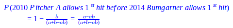
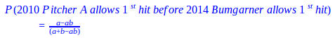
The first formula we construct determines the probability that 2010 Pitcher A will allow m hits before 2014 Bumgarner allows his 1^st hit; it is possible for the m^th hit from A and the 1^st hit from Bumgarner to occur after the same number of batters, but in a duel we want a clear winner. Let a be P(H) for 2010 Pitcher A and be a random variable for the total batters faced when he allows his m^th hit; similarly, let b be P(H) for 2014 Bumgarner and be a random variable for the total batters faced when he allows his 1^st hit. If 2010 Pitcher A allows his m^th hit on the j^th batter, he will have a combination of m hits and (j-m) non-hits (outs, walks, sacrifice flies, hit-by-pitches) with the respective probabilities of a and (1-a); meanwhile 2014 Bumgarner will eventually allow his 1^st hit on the (j+1)^th batter or later and he will have 1 hit and the rest non-hits with the respective probabilities of b and (1-b). We can then sum each j^th scenario together for any number of potential batters faced (all j≥m) to create the formula below:

If we assume an even pitchers’ duel of who will allow the 1^st hit, for m=1, then we have the following intuitive formula for 2010 Pitcher A versus 2014 Bumgarner:

This formula takes the probability that 2010 Pitcher A allows a hit minus the probability that both pitchers allow a hit and divides it by the probability that 2010 Pitcher A or 2014 Bumgarner allow a hit. Furthermore, if we let this happen for m hits, we arrive at our deduced formula. We should also note that according to the deduced formula, we should see the probability decrease as m increases. This logic makes sense because the expected span of batters until 2014 Bumgarner allows his 1^st hit, , stays the same, but we are trying to squeeze in more hits allowed by 2010 Pitcher A, which makes the probability become less likely.

Table 4.1:  Probability of 2010 Pitcher A Allowing m^th Hit Before 2014 Bumgarner Allows 1^st

In Table 4.1, we compare 2014 Bumgarner and his 0.123 World Series P(H) versus each starter from the 2010 World Series Giants rotation and their respective P(H). We expect 2014 Bumgarner to have the advantage over 2010 Lincecum, Cain, and Sanchez, given how he dominated the 2014 World Series; clearly he does. In an even pitchers’ duel, he would win with a probability greater than 50% even after the chance of a tie is removed; we could even see 2 hits from the other pitchers before 2014 Bumgarner allows his 1^st with a probability greater than 25%. However, against a comparably excellent pitcher, himself in 2010, he would likely lose the duel because 2010 Bumgarner actually has a better P(H). Notice that from Sanchez to Lincecum and from Lincecum to Cain, the P(H) descends steadily each time; consequently, the same pattern of linear decline also follows duel probabilities when transitioning from pitcher to pitcher for each of the different hits allowed. Hence, the distinction between exceptional and below-average pitchers stays relatively constant as we allow more hits by them versus 2014 Bumgarner.

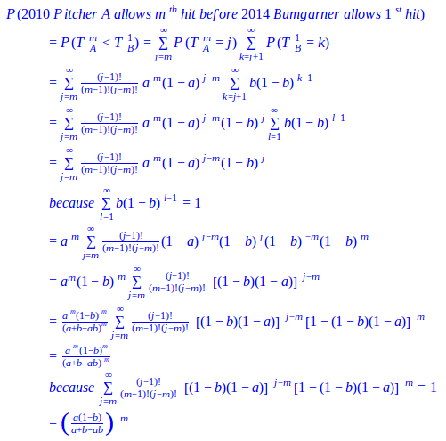
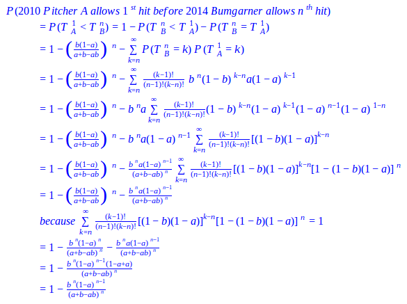
We can also construct the converse formula to calculate the probability that 2010 Pitcher A allows 1 hit before 2014 Bumgarner allows his n^th hit. We let be a random variable for the total batters faced when 2014 Bumgarner allows his n^th hit and for when 2010 Pitcher A allows his 1^st hit. However, instead of directly deducing the probability that 2010 Pitcher A allows 1 hit before 2014 Bumgarner allows his n^th hit, we’ll do so indirectly by taking the complement of both the probability that 2014 Bumgarner allows his n^th hit before 2010 Pitcher A allows his 1^st hit (a variation of our first formula) and the probability that 2014 Bumgarner allows his n^th hit and 2010 Pitcher A allows his 1^st hit after the same number of batters.

The resulting formula takes the complement of the probability that 2014 Bumgarner allows n hits and 2010 Pitcher A does not allow a hit in (n-1) chances and divides it by the probability that 2010 Pitcher A or 2014 Bumgarner allow n hits. In this formula we can contrarily see the probability increase as n increases. By extending the expected span of batters, , to accommodate 2014 Bumgarner’s n hits instead of just 1, we’re granting 2010 Pitcher A more time to allow his 1^st hit, resulting in an increased likelihood.

Once again, if we set n=1 for an even matchup, we get the same formula as before:

Table 4.2:  Probability of 2010 Pitcher A Allowing 1^st Hit Before 2014 Bumgarner Allows n^th

In Table 4.2, we again use 2014 Bumgarner’s 0.123 P(H) versus those displayed in the table above. As expected, the probabilities from the even duels are the same as Table 4.1 because the formulas are the same. Although this time from Sanchez to Lincecum and from Lincecum to Cain, the difference between each pitcher noticeably decreases as we adjust the scenario to allow 2014 Bumgarner more hits. Thereby, there is less distinction between exceptional and below-average pitchers if we widen the range of batters, , enough for them to allow their 1^st hit versus 2014 Bumgarner.

Madison Bumgarner may have dominated the 2014 World Series as a starter, but he also forcefully shut the door on the Royals to carry his team to the title (by ominously throwing 5 IP, 2 H, 0 BB). Given the momentum he had, he proved himself to be Bruce Bochy’s best option. However, not every game is Game 7 of the World Series, where a manager must decisively bring in the one reliever he trusts the most. A manager needs to assess who is the appropriate reliever for the job and weigh which relievers will available later. Fortunately, an indirect benefit of the pitchers’ duel model is that it can calculate the relative probability between two relievers for who will allow a hit or baserunner first; this application could be very useful in long relief or in extra innings.

Table 4.3:  Probability of 2010 Pitcher A Allowing m^th Baserunners Before 2014 Bumgarner Allows 1^st

Suppose we’re entering extra innings and the only pitchers available are 2014 Bumgarner and 2010 Bumgarner, Lincecum, Cain, and Sanchez with their respective statistics from Table 4.3 (where we substituted P(H) in Table 4.1 for OBP). We wouldn’t automatically throw in our best pitcher, 2014 Bumgarner, with his 0.151 OBP; we need to compare how he would perform relative to the other 2010 pitchers and see what the drop off is. Nor is it a priority to know how many innings to expect out of our reliever because we don’t know how long he’ll be needed. What is crucial in this situation is the prevention of baserunners as potential runs. 2010 Bumgarner, Cain, and Lincecum would each be worthy candidates to keep 2014 Bumgarner in the bullpen, because each has a reasonable chance (greater than 40%) of allowing a baserunner by the same batter or later than 2014 Bumgarner. Hence, the risk of using a pitcher with a slightly greater chance of allowing a baserunner sooner may be worth the reward of having 2014 Bumgarner available in a more dire situation. Yet, we would want to avoid bringing in 2010 Sanchez because the risk would be too great; the probability is approximately 49% that he could allow two baserunners before 2014 Bumgarner allows one. Preventing baserunners and using your bullpen appropriately are both high priorities in close game situations where mistakes are magnified.

This is installment 2 of the Player Evaluator and Calculated Expectancy (PEACE) system, which will culminate in a completely independent calculation of wins relative to replacement-level players.  Part 1 can be found here: http://www.fangraphs.com/community/an-introduction-to-calculated-runs-expectancy/

I reference Calculated Runs Expectancy a lot, so I highly recommend reading that article to gain some understanding of what I’m talking about.  Today I’m going to introduce my own defensive metric, zDefense, which operates under the same aggregate sum logic as UZR, but utilizes completely different arrangements of its components.

zDefense has 3 different methods of calculation: one for pitchers and catchers, one for infield positions, and one for outfielders.  I’ll explain how all three forms work to calculate each player’s defensive contribution in terms of runs relative to average (which for fielding is also considered “replacement-level”).  For this report, the seasons 2012-2014 have been calculated and will be compared throughout.

For pitchers and catchers, where Ball in Zone (BIZ) data isn’t available, the only calculation is zFielding, which measures how many relative runs player’s allowed according to Calculated Runs Expectancy (CRE).  For the pitchers, their defense is measured in terms of stolen bases, caught stealing, pickoffs, errors, and balks.  The catchers are judged based on stolen bases, caught stealing, wild pitches and passed balls, pickoffs, and errors.  In order to isolate each player’s individual contribution, each team’s “Base CRE” is calculated by taking their opponents’ offensive numbers and zeroing all baserunning/fielding statistics.  Then each player’s defensive numbers are included as the offensive counterpart and the difference between the new CRE calculation and the Base CRE indicates runs credited to that player defensively.  For example, in 2014 the St. Louis Cardinals had a Base CRE of 491 runs.  When analyzing Yadier Molina, his statistics (21 Stolen Bases, 23 Caught Stealing, 6 Pickoffs, 27 Bases Taken) are included in the equation and produce a new CRE value of 500, which means that he was responsible for about 9 runs allowed defensively.  This is done for all players and then compared to the positional average, which is where pitchers and catchers deviate from the other positions.

Without BIZ data, pitchers and catchers are evaluated based on the positional average number of innings played per defensive run allowed.  All other positions, however, are evaluated relative to the average number of runs allowed per ball in zone.  These numbers are almost constant year-to-year, with only miniscule variations (for example, the number of runs per BIZ for outfielders from 2012-2014 were 0.079, 0.079, and 0.078).

So in order to calculate Yadier Molina’s 2014 zDefense, his numbers would be plugged into the equation:

• zDefense (Pitchers/Catchers) = (Innings Played / Positional Innings per Run) – Player Defensive Runs Allowed

• zDefense (Molina, 2014) = (931.7 / 38.9) – 9.1 = +14.820

In 2014, catchers averaged one defensive run allowed every 38.9 innings; which means that an average catcher would be expected to allow about 24 runs in the number of innings that Molina caught.  Instead, he only allowed 9, saving the Cardinals nearly 15 runs in 2014.  This is all it takes to calculate the defensive contribution of pitchers and catchers.

For infielders and outfielders, zFielding is just one component; one that essentially tells how well fielders handled balls hit to them in terms of errors and preventing baserunner advancement.  It’s calculated slightly differently than for pitchers and catchers, but the first few steps are the same: find the team Base CRE, include player defensive stats, find the difference between the two CRE calculations, compare to positional rate.  Let’s use the Royals’ Alex Gordon in 2014 as an example.  The Royals as a team had a Base CRE of 519, and Gordon’s defensive contribution resulted in a new CRE of 528 (a difference of 9.1).  From here, just plug in the variables:

•  zFielding (Infielder/Outfielders) = (Positional Runs per BIZ * Player BIZ) – Player Defensive Runs Allowed

• zFielding (Gordon, 2014) = (0.064 * 261) – 9.1 = +7.724

Considering the number of balls in Gordon’s zone in 2014, he saved the Royals nearly 8 runs just by preventing errors and baserunner advancement.  But there are still a few other considerations for position players: zRange, zOuts, and zDoublePlays.

zRange attempts to quantify the number of runs saved by simply reaching balls in play using BIZ data and the runs per BIZ table from above.  It has 2 forms, one each for infielders and outfielders, but both begin the same way.  The first step is to find each position’s Real Zone Rating (RZR), which measures the percentage of BIZ fielded.  These numbers are more dynamic than the previous table, and the general trend has been towards higher RZR at all positions as offensive production has dwindled in the past decade.

The next step is basically the exact same as zFielding, except instead of finding relative runs allowed, we are looking for relative plays made.  For example, Alex Gordon in 2014 fielded 235 out of 261 BIZ (0.900 RZR), which was better than his positional average of 0.884.  By multiplying 261 and 0.884, it can be seen that Gordon reached about 4 more balls than the average left fielder would have.  From there, the relative number of plays is multiplied by the appropriate constant.  This is where one of the alterations to zDefense occurred.

For infielders, the idea is that by reaching a ball in play, the fielder has prevented the ball from reaching the outfield.  So in theory, this reduces the average number of runs that hit ball would be worth.  This is known as the IF (infield) Constant, and is the difference between the average runs per BIZ between outfield and infield balls in play.  In 2014 this constant was 0.068 (0.078 – 0.010), and has been nearly identical for each of the past three seasons.

For outfielders, the ball in play will almost always be classified as an outfield ball regardless of whether the fielder reaches it or not, so the OF (outfield) constant is just the average number of runs per BIZ for the outfield as a whole.  In 2014 this was 0.078, which would be multiplied by Gordon’s 4 relative plays above average.

Additionally, each player fields a number of balls outside of their zone (OOZ).  The number of OOZ plays is halved because they aren’t necessarily run-saving plays: when a shortstop catches a popup on the pitcher’s mound or when the first baseman extends to his right rather than let the second baseman handle the play, they may count as OOZ plays without being marginally beneficial.  The half of OOZ plays is also multiplied by the appropriate constant, added onto the previous product, and produces zRange.

• zRange = {[Player Plays Made – (Player BIZ * Positional RZR)] + (Player OOZ Plays Made / 2)} * IF/OF Constant

• zRange (Gordon, 2014) = {[235 – (261 * 884)] + (106 / 2)} * 0.078 = +4.436

On top of saving the Royals 8 runs with his arm and glove, Gordon also saved them over 4 runs with his legs and eyes.  This is where the biggest change to the formula happened; before, zRange was being calculated nearly identically to zOuts, which resulted in players essentially being credited twice with their relative RZR.  Instead, zRange just multiplies relative plays by the appropriate constant and recognizes that zOuts is a reflection of range and ability to convert balls into outs.

zOuts uses a very different approach than the previous 2 components; rather than find relative run values by conventional means, a rate statistic z-score is found and then multiplied by “playing time.”  It will be shown in the next section that this works remarkably well, but for now we are just looking at the derivation.  For zOuts, 2 different numbers are required for each player: their Real Zone Rating, and their Field-to-Out Percentage (F2O%).  These 2 numbers combine to form outs per BIZ, which is the comparative average each player is evaluated against.  Like the previous numbers, these also remain fairly consistent with a general trend negatively related to scoring.

Also required for z-scores is the standard deviation.  For these calculations, I have been using the standard deviation for just players with at least 100 innings played at that position to eliminate outliers.

Taking the z-score of outs per BIZ is simple enough, but what defines “playing time?”  Well, there are 2 factors that work well in eliminating outliers: the first is the percentage of total innings played at that position by that player.  If a team plays 1400 innings in the field over the course of the year, it means there are 1400 defensive innings available at each position, so a player who played in 1000 of them would have played about 71% of the defensive innings at that position.  The second factor considers that while players may have played an equal number of innings, they may not have had an equal number of balls to field.  This factor is one-half the square root of the number of BIZ for each player.

• zOuts = [(Player O/BIZ – Positional O/BIZ) / Positional O/BIZ Standard Deviation] * (Player Innings / Team Innings) * (√ Player BIZ / 2)

• zOuts (Gordon, 2014) = [(0.450 – 0.417) / 0.068] * (1372.7 / 1450.7) * (√ 261 / 2) = +3.741

zOuts is a blended statistic; it measures how well players convert balls into outs by considering their range and out-producing ability.  Alex Gordon saved the Royals another 4 runs this way, which brings his total zDefense to:

• zDefense (Outfielders) = zFielding + zRange + zOuts

• zDefense (Gordon, 2014) = +7.724 + 4.436 + 3.741 = +15.900

This is all it takes to calculate the defensive contribution of outfielders, but infielders still have one more factor to consider: double play ability.  zDoublePlays is nearly identical to zOuts, except double plays per BIZ is the positional average required.

From there, the calculation is almost the same as zOuts:

• zDoublePlays = [(Player DP/BIZ – Positional DP/BIZ) / Positional DP/BIZ Standard Deviation] * (Player Innings / Team Innings) * (√ Player BIZ / 2) * Positional DP/BIZ

The last part at the end affects the weight of zDP in the overall zDefense equation.  The ability to turn double plays isn’t really a selling point for corner infielders because of the relative rarity of those plays.  Double play ability is much more relevant to middle infielders, and multiplying by the positional averages helps to bring this disparity into the equation.  JJ Hardy consistently ranks as elite in terms of double play ability, so we’ll use him as the example player here:

• zDoublePlays (Hardy, 2014) = [(0.313 – 0.236) / 0.091] * (1257.0 / 1461.3) * (√ 316 / 2) * 0.236 = +1.540

And if we want the entire infielder formula written out:

• zDefense (Infielders) = zFielding + zRange + zOuts +zDoublePlays

Like the previous post, there is a lot of new information to take in here, so feel free to ask any questions or leave any comments with feedback, thoughts, or concerns with work I’ve presented.  The next installment will be an exploration of z-scores in sports and how they correspond to actual points/runs, which I’ll use to provide credibility for zDefense.

Introduction first: my name is Walter King and over the next few weeks I plan on sharing my counter to Wins Above Replacement, which I call PEACE: Player Evaluator and Calculated Expectancy.  The engine behind PEACE is Calculated Runs Expectancy, which is what this article will cover.

Calculated Runs Expectancy (CRE) is an analytical model that estimates runs produced by a player, team, or league for any number of games.  CRE operates under the assumption that every single play on the field is relevant to output and thus can be translated into a statistical measure.

In its general form, the Calculated Runs Expectancy formula looks like this:

•  CRE = (√ {[(Bases Acquired) * [(Potential Runs) * (Quantified Advancement) / (Total Opportunities)]] / Outs Made²} * (Total Opportunities) + (Hit and Run Plays) + Home Runs) / Runs Divisor, relative to the league

This formula was reached by following a particular line of logical reasoning, which starts with the assumption that the singular objective of baseball is to win every game (well, duh!).  Winning every game mathematically requires one of two scenarios: either a team allows zero runs, or they score an infinite number of runs, both resulting in one team scoring 100% of the runs, assuring 100% of the wins.  Because the objective is to win the game, and the only way to assure victory is to score the most runs, then the only two ways players can contribute to winning are by scoring runs or by preventing the opponent from doing so.  This sounds painfully simple, but we have to establish that metrics are limited in usefulness if there is no clear link to runs, and therefore wins.  This assumption forces us to define what makes a run in terms of statistics.

With so many different statistics to represent the happenings on the field, it can be tough to form a clear definition.  Keep it simple.  Break down what a run is in the simplest way possible: a run scored is when a player safely touches all four bases, ending by touching home plate.  That’s it.  A team must acquire at least 4 bases in order to score 1 run, so the first formula we can use in our analysis is Bases Acquired:

•  Bases Acquired = TB + BB + HBP + ROE + XI + SH + SF + SB + BT (bases taken)

This is a complete representation of the number of individual bases a hitter acquired, which is often overlooked as valuable information.

My second definition of a run comes directly from Bill James’ Runs Created statistic: to  score a run, a batter needs to first reach base, and then advance among the bases until they reach home plate.  This focus looks at offensive production through the completion of those two smaller goals.  These concepts have already been identified by James using three basic principles: On-Base Factor, Advancement Factor, and Opportunity Factor to calculate runs created.

But what composes these factors?  Well, this is where I venture slightly away from James, attempting to encompass a more complete representation of a hitter in my calculations.  I’ve altered them a bit and given them new names:

• Potential Runs = TOB (times on base) – CS – GDP – BPO (basepath outs)
• Quantified Advancement = TB + SB + SH + SF + BT
• Total Opportunities = PA + SB + CS + BT + BPO

With these now defined, my modified Runs Created formula looks like this:

•  Modified Runs Created = [(TOB – CS – GIDP – BPO) * (TB + SB + SH + SF + BT)] / (PA + SB + CS + BT + BPO)

Bases Acquired and Runs Created are counting statistics, but we want rate statistics.  I believe strongly in the principles of VORP, which asserts that production must always be measured relative to cost in terms of outs.  To amalgamate our measures of offensive production and outs made, we simply divide each by outs made to create two “per out” statistics.

So what we have now are two different measures of a batter’s efficiency; one that calculates bases acquired per out made and another that finds calculated runs scored per out made.  By multiplying the two, we can incorporate two different statistics of efficiency in our evaluation of hitters.  Conceptually, this represents a reconciliation of two different philosophies on how runs are produced.  We’ll call the resulting quantity Offensive Efficiency.

•  Offensive Efficiency = (Bases Acquired * Runs Created) / Outs Made²

I particularly like this formula because the two key components that comprise it are largely considered obsolete by modern sabermetrics.  Both Total Average (bases/outs) and Runs Created are from the 1970s and are throwbacks to better uniforms and simpler ways of thinking.  If you were to approach a stathead today championing total average or runs created as “the answers,” they would first dismiss you, and then suggest more modern metrics.  Much like the struggle sabermetrics saw when first attempting to become a respected pursuit, modern sabermetrics seems to scoff at the idea that older, simpler calculations can be valuable.  But both Total Average and Runs Created per Out are logically sound in their function; they break down the aspects of hitting into real-life objectives that correspond to real-life results.  Offensive Efficiency will definitely tell you which batters performed most efficiently, but it is sensitive to outliers.  To counter this, recall the general CRE equation:

•  CRE = (√ {[(Bases Acquired) * [(Potential Runs) * (Quantified Advancement) / (Total Opportunities)]] / Outs Made²} * (Total Opportunities) + (Hit and Run Plays) + Home Runs) / Runs Divisor, relative to the league

Multiplying Offensive Efficiency by Total Opportunities creates a balance between efficient and high-volume performers.  The next step, inspired by Base Runs, is to add “Hit and Run Plays” along with Home Runs to the equation because those are instances when a run is guaranteed to score.  Hit and Run Plays are my name for situational baserunning plays (found on Baseball-Reference) that result in a batter advancing more bases than the ball in play would suggest.  For example, when a batter hits a single with a runner on first, the runner would be definitely expected to reach second base.  Reaching third or scoring, however, would indicate a skillful play (or a hit and run) by an opportunistic baserunner.  Three stats make up Hit and Runs Plays: 1s3/4 (reaching third or home from first on a single), 2s4 (scoring from second on a single), and 1d4 (scoring from first on a double).

At this point, all that’s left is the Runs Divisor.  If you’re following along at home, an individual batter season without a Runs Divisor would be somewhere between 200-500, while a team single season would typically be between 2000-3000.  The Runs Divisor is specific to each season and league (so the 2014 AL and NL both have unique divisors), and is the average optimal divisor that would result in actual runs scored, relative to the specific league.  Let’s use a 2-team league as an example.  Team A scores a raw CRE of 2500 while scoring 700 actual runs, so their optimal divisor would be 3.57.  Team B, on the other hand, has a raw CRE of 2250 and scored 600, a divisor of 3.75.  The league’s Runs Divisor would be the average of the two: 3.66.  This divisor would be used for every individual player in that league, as well.  Divisors vary every year, but always remain very similar.

A full list of Runs Divisors from the seasons 1975-2014 can be seen here:

The average divisor across that time span was 3.7631, with a standard deviation of just 0.0268.  This provides strong evidence of the relationship between CRE and runs; the two are related in the same way across generations of ballplayers.  When we graph the results of CRE against actual runs for all 1114 teams in that timespan, we can see some very convincing results:

The R2 value (0.9682) corresponds to an average difference between actual and calculated runs of 14.02.  When compared to other run estimators, the differences are significant:

Runs Estimator (Creator), Average, R2

• Base Runs (David Smyth), 18.77, 0.9441             
• Estimated Runs Produced (Paul Johnson), 18.15, 0.9480             
• Extrapolated Runs (Jim Furtado), 18.33, 0.9515             
• Runs Created (Bill James), 20.01, 0.9383                         
• Weighted Runs Created (Tom Tango), 19.37, 0.9443  

The gap between CRE and the 5 other estimators is consistent across the entire span of 40 seasons.

There is a lot of new information to take in here, so feel free to comment below with any questions or feedback.  Part 2 will be uploaded in a few days.

If you read or surf through once in a while, you will surely venture across baseball job openings. It is enlightening to see an increasing amount of analytics positions looking to be filled, especially with major league teams. Advanced stats and sabermetrics have emerged in the last decade. This is clear. What is not clear yet is if the once niche perspective is fully sunk into mainstream baseball culture. Certainly, this wasn’t true a couple years ago, or Mike Trout’s MVP award would not be his only one.

It would be a lie to say that advanced statistics have been beyond the peripherals in major award voting in recent years. I am fairly certain that a league leading ERA and WHIP were not enough to win an AL Cy Young award this past season (poor Felix). Not to mention that the same Mariner took home the glory with a murky 13-12 record a few years ago. On the Gold Glove circuit, I can make the open claim that defensive metric leaders and Gold Glove victors lined up much more this year than they have in the past. Even Adam Jones’ defensive season was arguably deserving of a gold glove (not his 4^th though…).

Let us focus on baseball’s best player (I can say that now, right?). Mike Trout has been juiced out of at least one MVP, and maybe two depending on what side of the fence you sit. From the table below you can see his “traditional” stats in both those years.

From analyzing the first table, he still had fantastic years. And as we know, he scored back-to-back 10 fWAR seasons. On the other hand, here is what Miguel Cabrera’s corresponding numbers look like:

Based on the tables, the main drivers year over year seem to be home runs and RBI. From 1993 to 2007, every single AL MVP had 30 homers and 100 RBI – aside from leadoff hitting Ichiro in 2001. In the NL, the song remains the same with only Barry Larkin failing to reach the 30 homer mark and two others merely totalling 90+ RBI. While this was a steroid heavy era, there is not enough reason to discredit the data, as with an even larger sample of MVPs, the same trends can be drawn. In 2012, Miguel’s “box” looks significantly better – 137 to 83 RBI is quite a large gap. To avoid sounding like a broken record, I will not mention the poor defense and baserunning that the Tigers corner infielder accounted for. That is why Trout’s standalone fWAR numbers are second to none. In 2013, it was more of the same from Trout. The 10 fWAR season was almost double Cabrera’s, but a 179 OPS+ (park- and league-adjusted) put him behind Cabrera’s 190 OPS+. With the defense and baserunning, it was still likely another Trout miss by the voters.

Arriving back to present time with Trout holding his trophy, it is worth understanding what he did differently. In short, he started being more aggressive and his whiff rate (number of swings and misses per pitch) rose. I would also speculate that with Statcast data, we would see ball speed off his bat is faster this year. As for his results, there is no surprise his strikeout rate jumped, nor is there for the home run total. As they positively correlate, the RBI came up too, leaving his “traditional” numbers looking like this. His fWAR total is also alongside.

While it is common on a typical defense and baserunning aging curve, the former and the latter did, in fact, take dives as well this year. Trout’s willingness to run decreased by more than 50% (18 total stolen base attempts) and he actually graded out as a relatively bad center fielder.

My claim here is simple. Mike Trout, whether acting purposeful or not, did what the classic MVP voting criteria wanted him to do – hit homers and drive in runs. This past season, Trout was significantly less valuable than he was in his previous two years, but according to the traditional measures, he was fabulous in the now hitting-depressed baseball. In September of 2012, Trout was quoted saying “I was trying to do too much, trying to hit home runs when I shouldn’t be.” Clearly, he has discarded this mentality, and because of it, he unanimously captured the MVP – the first American Leaguer to do so since Ken Griffey Jr. in 1997.

Can you see the irony here? Mike Trout manages two consecutive 10 fWAR seasons, a feat only done by Barry Bonds, Willie Mays and Mickey Mantle. He doesn’t win the MVP in either one. The next year he cuts his fWAR by almost 3 wins but adds 28 RBI and half a dozen homers to his totals. All of the foregoing occurs, in the era in which sabermetrics are undoubtedly now integrated into modern baseball. (Fortunately for him, he didn’t need 10 WAR to be seen as baseball’s best player). The fact is that Mike Trout just won the MVP – the traditional way.

(This is Part 2 of a four-part series answering common questions regarding starting pitchers by use of discrete probability models.  In Part 1, we dealt with the probability of a perfect game or a no-hitter. Here we deal with the other hit probabilities in a complete game.)

III. Yes! Yes! Yes, Hitters!

Rare game achievements, like a no-hitter, will get a starting pitcher into the record books, but the respect and lucrative contracts are only awarded to starting pitchers who can pitch successfully and consistently. Matt Cain and Madison Bumgarner have had this consistent success and both received contracts that carry the weight of how we expect each pitcher to be hit. Yet, some pitchers are hit more often than others and some are hit harder. Jonathan Sanchez had shown moments of brilliance but pitch control and success were not sustainable for him. Tim Lincecum had proven himself an elite pitcher early in his career, with two Cy Young awards, but he never cashed in on a long term contract before his stuff started to tail off. Yet, regardless of success or failure, we can confidently assume that any pitcher in this rotation or any other will allow a hit when he takes the mound. Hence, we should construct our expectations for a starting pitcher based on how we expect each to get hit.

An inning is a good point to begin dissecting our expectations for each starting pitcher because the game is partitioned by innings and each inning resets. During these independent innings a pitcher’s job is generally to keep the runners off the base paths. We consider him successful if he can consistently produces 1-2-3 innings and we should be concerned if he alternately produces innings with an inordinate number of base runners; whether or not the base runners score is a different issue.

Let BR be the base runners we expect in an inning and let OBP be the on-base percentage for a specific starting pitcher, then we can construct the following negative binomial distribution to determine the probabilities of various inning scenarios:

If we let br be a random variable for base runners in an inning, we can apply the formula above to deduce how many base runners per inning we should expect from our starting pitcher:

The resulting expectation creates a baseline for our pitcher’s performance by inning and allows us to determine if our starting pitcher generally meets or fails our expectations as the game progresses.

Table 3.1: Inning Base Runner Probabilities by Pitcher

Based upon career OBPs through the 2013 season, Bumgarner would have the greatest chance (0.356) of retiring the side in order and he would be expected to allow the fewest base runners, 1.233, in an inning; Cain should also have comparable results. The implications are that Bumgarner and Cain represent a top tier of starting pitchers who are more likely to allow 0 base runners than either 1 base runner or +2 base runners in an inning. A pitcher like Lincecum, expected to allow 1.326 base runners in an inning, represents another tier who would be expected to pitch in the windup (for an entire inning) in approximately ⅓ of innings and pitch from the stretch in ⅔ of innings. Sanchez, on the other hand, represents a respectively lower tier of starting pitchers who are more likely to allow 1 or +2 base runners than 0 base runners in an inning. He has the least chance (0.280) of having a 1-2-3 inning and would be expected to allow more base runners, 1.586, in an inning.

As important as base runners are for turning into runs, the hits and walks that make up the majority of base runners are two disparate skills.  Hits generally result from pitches in the strike zone and demonstrate an ability to locate pitches, contrarily, walks result from pitches outside the strike zone and show a lack of command.  Hence, we’ll create an expectation for hits and another for walks for our starting pitchers to determine if they are generally good at preventing hits and walks or prone to allowing them in an inning.

Let h, bb, and hbp be random variables for hits, walks, and hit-by-pitches and let P(H), P(BB), P(HBP) be their respective probabilities for a specific starting pitcher, such that OBP = P(H) + P(BB) + P(HBP). The probability of Y hits occurring in an inning for a specific pitcher can be constructed from the following negative multinomial distribution:

We can further apply the probability distribution above to create an expectation of hits per inning for our starting pitcher:

For walks, we do not have to repeat these machinations.  If we simply substitute hits for walks, the probability of Z walks occurring in an inning and the expectation for walks per inning for a specific pitcher become similar to the ones we deduced earlier for hits:

We could repeat the same substitution for hit-by-pitches, but the corresponding probability distribution and expectation are not significant.

Table 3.2: Inning Hit Probabilities by Pitcher

The results of Table 3.2 and Table 3.3 are generated through our formulas using career player statistics through 2013. Cain has the highest probability (0.466) of not allowing a hit in an inning while Sanchez has the lowest probability (0.439) among our starters. However, the actual variation between our pitchers is fairly minimal for each of these hit probabilities. This lack of variation is further reaffirmed by the comparable expectations of hits per inning; each pitcher would be expected to allow approximately 0.9 hits per inning. Yet, we shouldn’t expect the overall population of MLB pitchers to allow hits this consistently; our the results only indicate that this particular Giants rotation had a similar consistency in preventing the ball from being hit squarely.

Table 3.3: Inning Walk Probabilities by Pitcher

The disparity between our starting pitchers becomes noticeable when we look at the variation among their walk probabilities. Bumgarner has the highest probability (0.776) of getting through an inning without walking a batter and he has the lowest expected walks (0.264) in an inning. Sanchez contrarily has the lowest probability (0.589) of having a 0 walk inning and has more than double the walk expectation (0.580) of Bumgarner. Hence, this Giants rotation had differing abilities targeting balls outside the strike zone or getting hitters to swing at balls outside the strike zone.

Now that we understand how a pitcher’s performance can vary from inning to inning, we can piece these innings together to form a 9 inning complete game. The 9 innings provides complete depiction of our starting pitcher’s performance because they afford him an inning or two to underperform and the batters he faces each inning vary as he goes through the lineup. At the end of a game our eyes still to gravitate to the hits in the box score when evaluating a starting pitcher’s performance.

Let D, E, and F be the respective hits, walks, and hit-by-pitches we expect to occur in a game, then the following negative multinomial distribution represents the probability of this specific 9 inning game occurring:

Utilizing the formula above we previously answered, “What is the probability of a no-hitter?”, but we can also use it to answer a more generalized question, “What is the probability of a complete game Y hitter?”, where Y is a random variable for hits. This new formula will not only tell us the probability of a no-hitter (inclusive of a perfect game), but it will also reveal the probability of a one-hitter, three-hitter, etc. Furthermore, we can calculate the probability of allowing Y hits or less or determine the expected hits in a complete game.

Let h, bb, hbp again be random variables for hits, walks, and hit-by-pitches.

The derivations of the complete game formulas above are very similar to their inning counterparts we deduced earlier. We only changed the number of outs from 3 (an inning) to 27 (a complete game), so we did not need to reiterate the entire proofs from earlier; these formulas could also be constructed for an 8 inning (24 outs), a 10 2/3 inning (32 outs), or any other performance with the same logic.

Table 3.4: Complete Game Hit Probabilities by Pitcher using BA

The results of Table 3.4 were generated from the complete game approximation probabilities that use batting average (against) as an input. Any of the four pitchers from the Giants rotation would be expected to allow 8 or 9 hits in a complete game (or potentially 40 total batters such that 40 = 27 outs + 9 hits + 4 walks), but in reality, if any of them are going to be given a chance to throw a complete game they’ll need to pitch better than that and average less than 3 pitches per batter for their manager to consider the possibility. If we instead establish a limit of 3 hits or less to be eligible for a complete game, regardless of pitch total, walks, or game situation (not realistic), we could witness a complete game in at most 1 or 2 starts per season for a healthy and consistent starting pitcher (approximately 30 starts with a 5% probability). Of course, we would leave open the possibility for our starting pitcher to exceed our expectations by throwing a two-hitter, one-hitter, or even a no-hitter despite the likelihood. There is still a chance! Managers definitely need to know what to expect from their pitchers and should keep these expectations grounded, but it is not impossible for a rare optimal outcome to come within reach.

I’ve often wondered if some sort of bizarre connection exists between names and athletic ability, specifically when it comes to the sport of baseball. Considering I grew up in the 90’s, I will always associate certain names with possessing a supreme baseball talent. Names like Ken (Griffey Jr.), Mike (Piazza), Randy (Johnson), Greg (Maddux) and Frank (Thomas) are just a few examples. With a wealth of statistical information available, I thought I’d investigate into the possibility of an abnormal association between names and baseball skill.

I began digging up the most popular given names, by decade, using the 1970’s, 80’s & 90’s as focal points. This information was easily accessible on the official website of the U.S. Social Security Administration, as they provide the 200 most popular given names for male and female babies born during each decade. After scouring through all of the names listed, the records revealed there were 278 unique names appearing during that timespan.

Having narrowed down the most popular names for the timeframe, I wandered over to FanGraphs.com, to begin compiling the “skill” data. I will be using the statistic known as WAR (Wins Above Replacement) as my objective guide for evaluating talent. Sorting through all qualified players from 1970-1999, the data revealed 2,554 players eligible for inclusion. After combining all full names with their corresponding nicknames (i.e.: Michael & Mike), the list was condensed down to 507 unique names.

By comparing the 278 unique names identified via the Social Security Administration’s most popular names data, with the 507 qualified ballplayer names collected through FanGraphs, it was discovered that 193 of the names were present on both lists. The following tables point out some of the more intriguing findings the research was able to provide.

The first table[Table 1], below, is comprised of the 25 most frequent birth names from 1970-1999. The second table[Table 2] consists of the 25 WAR leaders by name, meaning the highest aggregate WAR totals collected by all players with that name. Naturally, many of the names that appear in the 25 most common names list, reappear here as well. Ken, Gary, Ron, Greg, Frank, Don, Chuck, George and Pete are the exceptions. It’s interesting to see that these names seem to have a higher AVG WAR per 1,000 births(as seen on the final table), perhaps indicative of those names’ supremacy as better baseball names? The last table[Table 3] contains the top 25 names by AVG WAR per 1,000 births; here we see some less common names finally begin to appear. These names provide the most proverbial bang (WAR) for your buck (name). Yes, some names, like Barry and Reggie, are inflated in the rankings — probably due to the dominant play of Barry Bonds and Reggie Jackson, but could it not also mean these players were just byproducts of their birth names?!? Probably not, but it’s interesting, nonetheless.

So if you’re looking to increase the chances your child will make it professionally as a baseball player, then you might want to take a look at the names toward the top of the AVG WAR per 1,000 births table, choose your favorite, and hope for the best…OR, you could always just have a daughter.

Please post comments with your thoughts or questions. Charts can be found below.

25 Most Common Birth Names 1970-1999

25 Highest Cumulative WAR, by Name, 1970-1999

25 Highest WAR per 1,000 Births, by Name, 1970-1999

I’m mostly an NFL writer. For years, I’ve been naming an NFL All-Loser Team at the end of each regular season. It’s an all-star team comprised exclusively of players whose teams missed the postseason. You can view it as a celebration of players who may be underrated or underappreciated because their teams aren’t very good, or you can view it as a shot at people who insist you can’t be that great if your team didn’t make the playoffs. Up to you. It’s a fun project, and it’s easy to apply to MLB as well football.

Here’s what you’re getting after the jump:

* Four teams. We’ll do an American League All-Loser Team, National League All-Loser Team, MLB All-Loser Team, and an all-star team taken exclusively from the six clubs that finished last in their divisions.

* For each list, we’ll do nine position players (the NL gets a pinch-hitter instead of a DH), and I’ll show my imaginary batting order. Each team will also feature a five-man rotation, a right-handed reliever, and a left-handed reliever. So, 16 players per team.

* I’ll offer some minimal commentary on the teams, with a paragraph or two for each team to discuss surprising selections and close calls. For the MLB team, I’ll list the top three in fWAR at each position and explain my selections. There’s nothing earth-shattering here, unless you think we can’t make a wicked lineup out of players from losing teams.
Read the rest of this entry »