Examining the foundations of batting analysis began in Part 1 with an historical examination of the earliest statistics designed to examine the performance of batters. In Part 2, I presented a new method for calculating basic averages reflecting the “real and indisputable” rate at which batters reached base. In Part 3, I examined the development of run estimation techniques over the last century, culminating with the linear weights system. I will employ that system now as I reconstruct run estimation from the bottom up.

We use statistics in baseball to tell stories. Statistics describe the action of the game or the performance of players over a period of time. Statistics inform us of how much value a player provided or how much skill a player showed in comparison to other players. To tell such stories successfully, we must understand how the statistics we use are constructed and what they actually represent.

A single, for instance, seems simple enough at first glance. However, there are details in its definition that we sometimes gloss over. In general, a single is any event in which the batter puts the ball into play without causing an out, while showing an accepted form of batting effectiveness (reaching on a hit), and ultimately advancing to first base due to the primary action of the event (before any secondary fielding errors or advancement on throws to other bases). Though this is specific in many regards, it is still quite a broad definition for a batting event. The event could occur in any inning, following any number of outs, and with any number of runners on the bases. The ball could be hit in any direction, with any speed and trajectory, and result in any number of baserunners advancing any number of bases.

These kinds of details form the contextual backdrop that characterizes all batting events. When we construct a statistic to evaluate these events, we choose what level of contextual detail we want to consider. These choices define our analysis and are critical in developing the story we want to tell. For instance, most statistics built to measure batting effectiveness—from the simple counting statistics like hits and walks, to advanced run estimators like Batter Runs or weighted On Base Average (wOBA)—are constructed to be independent of the “situational context” in which the events occur. That is, it doesn’t matter when during the game a hit is made or if there are any outs or any runners on the bases at the time it happens. As George Lindsey noted in 1963, “the measure of the batting effectiveness of an individual should not depend on the situations that faced him when he came to the plate.”

Situational context is the most commonly cited form of contextual detail. When a statistic is described as “context neutral,” the context being removed is very often the one describing the out/base state before and after the event and the inning in which it occurred. However, there are other contextual details that characterize the circumstances and conditions in which batting events occur that also tend to be removed from consideration when analyzing their value. Historically, where the ball was hit, as well as the speed and trajectory which it took to reach that location, have also not been considered when judging the effectiveness of batters. This has partly been due to the complexity of tracking such things, especially in the century of baseball recordkeeping before the advent of computers. Also, most historical batting analyses focus exclusively on the outcome for the batter, independent of the effect on other baserunners. If the batter hits the ball four feet or 400 feet but still only reaches first base, there is no difference in the personal outcome that he achieved.

If the value of a hit was limited to only how far the batter advances, then there would be no need to consider the “batted-ball context,” but as F.C. Lane observed in 1916, part of the value of making a hit is in the effect on the “runner who may already be upon the bases.” By removing the batted-ball context when considering types of events in which the ball is put into play, we’re assuming that a four-foot single and 400-foot single have the same general effect on other baserunners. For some analyses, this level of contextual detail describing an event may be irrelevant or insignificant, but for others—particularly when estimating run production—such a level of detail is paramount.

Let’s employ the linear weights method for estimating run production, but allow the estimation to vary from one completely independent of any contextual detail to one as detailed as we can make it. In this way, we’ll be able to observe how various details impact our valuation of events. Also, in situations where we are only given a limited amount of information about batting events, it will allow us to make cursory estimations of how much they caused their team’s run expectancy to change.

To begin, let’s define the run-scoring environment for 2013.[i] While we have focused on context concerning how events transpired on the field, the run scoring environment is another kind of contextual detail that characterizes how we evaluate those events. The exact same event in 2013 may not have caused the same change in run expectancy as it would have in 2000 when runs were scored at a different rate. We will define the run scoring environment for 2013 as the average number of runs that scored in an inning following a plate appearance in each of the 24 out/base states – a 2013-specific form of George Lindsey’s run expectancy matrix:

While we will focus on examining various levels of contextual detail concerning the events themselves, the run-scoring environment can also be varied based on contextual details concerning the scoring of runs. The matrix we will employ, as defined by Lindsey, reflects the average number of runs scored across the entire league. If we wanted, we could differentiate environments by league or park, among other things, to try and reflect a more specific estimate of the number of runs produced. As the work I’m going to present is meant to provide a general framework for run estimation, and these adjustments are not trivial, I’m going to stick with the basic model provided by Lindsey.

With Lindsey’s tool, we can define a pair of statistics for general analysis of run production. Expected Runs (xR) reflect the estimated change in a team’s run expectancy caused by a batter’s plate appearances independent of the situational context in which they occur. A batter’s expected Run Average (xRA) is the rate per plate appearance at which he produces xR.

xRA = Expected Runs / Plate Appearances = xR / PA

xR and xRA create a framework for estimating situation-neutral run production. Based on the contextual specificity that is used to describe the action of a plate appearance, xR and xRA will yield various estimations. The base case for calculating expected runs, xR₀, is calculated independently of any contextual detail, considering only that a plate appearance occurred. By definition, an average plate appearance will cause no change in a team’s run expectancy. Consequently, no matter a player’s total number of plate appearances, his xR₀ and, by extension, his xRA₀, will be 0.0.

This is completely uninformative of course, as base cases often are. So let’s add our first layer of contextual specificity by noting whether an out occurred due to the action of the plate appearance. This is the most significant contextual detail that we consider when evaluating batting events – it is the only factor that determines whether a plate appearance increases or decreases a team’s run expectancy. In 2013, 67.5 percent of all plate appearances resulted in at least one out occurring. On average, those events caused a team’s run expectancy to decrease by .252 runs. The 32.5 percent of plate appearances in which an out did not occur caused a team’s run expectancy to increase by .524 runs on average. We’ll define xR₁ as the estimated change in run expectancy based exclusively on whether the batter reached base without causing an out; xRA₁ is the rate at which a batter produced xR₁ per plate appearance.

You’ll notice that the components that construct xRA₁ can only take on two values—.524 and -.252—in the same way that the components that construct effective On Base Average (eOBA) (as defined in Part 2) can only take on two values—1 and 0. These statistics—xRA₁ and eOBA—have a direct linear correlation:

In effect, xRA₁ is a weighted version of eOBA, incorporating the same contextual details but on a different scale. This estimation provides us with an association between reaching base safely and producing runs. However, the lack of detail would suggest that all players that reach base at the same rate produce the same value, which is over simplified. It’s why you wouldn’t just use eOBA, or eBA, or any other basic statistic that reflects the rate which a batter reaches base, when judging the performance of a batter. Let’s add another layer of contextual detail to account for the different kinds of value a batter provides when he reaches base.

xR₂ will represent the estimated change in run expectancy based on whether the batter safely reached base and the number of bases to which he advanced due to the action of the plate appearance; xRA₂ will be the rate at which a batter produces xR₂ per plate appearance. While xR₁ and xRA₁ were built with just two components to estimate run production, xR₂ and xRA₂ require five components: one to define the value of an out, and four to define the value of safely reaching each base.

In 2013, a batter safely reaching first base during a plate appearance caused an average increase of .389 runs to his team’s run expectancy. Reaching second base was worth .748 runs, third base was worth 1.026 runs, and reaching home was worth 1.377 runs on average. Where xRA₁ provided a run estimation analog to eOBA, xRA₂ is built with very similar components to effective Total Bases Average (eTBA), though it’s not quite a direct linear correlation:

The reason xRA₂ and eTBA do not correlate with each other perfectly, like xRA₁ and eOBA, is because the way in which a batter advances bases is significant in determining how valuable his plate appearances were. Consider two players that each had two plate appearances: Player A hit a home run and made an out, Player B reached second base twice. Their eTBA would be identical—2.000—as they each reached four bases in two plate appearances. However, from the run values associated with reaching those bases, Player A would record 1.125 xR₂ from his home run and out, while Player B would record 1.496 xR₂ from the two plate appearances leaving him on second base. Consequently, Player A would have produced a lower xRA₂ (.5625) than Player B (.7480), despite their having the same eTBA. These effects tend to average out over a large enough sample of plate appearances, but they will still cause variations in xRA₂ among players with the same eTBA.

As stated in Part 2, the two main objectives of batters are to not cause an out and to advance as many bases as possible. If the only value that batters produced came from accomplishing these objectives, then we would be done – xR₂ and xRA₂ would reflect the perfect estimations of situation-neutral run production. As I hope is clear, though, the value of a batting event is dependent not only on the outcome for the batter but on the impact the event had on all other runners on base at the time it occurred. Different types of events that result in the batter reaching the same base can have different average effects on other baserunners. For instance, a single and a walk both leave the batter on first base, but the former creates the opportunity for baserunners to advance further on average than the latter. To address this, the next layer of contextual detail will bring the official scorer into the fray. xR₃ will represent the estimated change in run expectancy produced during a batter’s plate appearance based on:

(1)    whether the batter safely reached base,

(2)    the number of bases, if any, to which the batter advanced due to the action of the plate appearance, and

(3)    the type of event, as defined by the official scorer, that caused him to reach base or cause an out.

xRA₃ will, as always, be the rate at which a batter produces xR₃ per plate appearance.

Each of the run estimators that were examined in Part 3, from F.C. Lane’s methods through wOBA, are subsets of this level of xR. Expected runs incorporate estimations of the value produced during every event in which the batter was involved, including those which may be considered “unskilled.” The run estimators examined in Part 3 consider only those events that reflected a batter’s “effectiveness,” and either disregard the “ineffective” events or treat them as failures. xR₃ provides the total value produced by a batter, independent of the effectiveness he showed while producing it, based solely on how the official scorer defines the events. Consequently, some events, like strikeouts, sacrifice bunts, reaches on catcher’s interference, and failed fielder’s choices, among other more obscure occurrences, are examined independently in xR₃. From the two components of xR₂ and the five of xR₃, we build xR₄ with 18 components: five types of outs and 13 types of reaches.

To help illustrate how xR has progressed from level to level, here is a chart reflecting the run values for 2013 as estimated by xR based on the contextual detail provided thus far.

xR Progression

Beyond any consideration of skilled or unskilled production, xR₃ is the level at which most run estimators are constructed. It incorporates events that are well defined in the Official Rules of the game, and have been for at least the last few decades, and in some cases for over a century. While we still define most of a batter’s production by his accomplishing these events, we live in an era where we can differentiate between events on the field in more specific ways. Not all singles are identical events. We weaken our estimation of run production if we don’t account for the different kinds of singles, among other events, that can occur. xR₃ brought the official scorer into action; xR₄ will do the same with the stat stringer.

While the scorer is concerned with the result of an event, a stringer pays attention to the action in between the results. They chart the type, speed, and location of every pitch, and note the batted ball type (bunt, groundball, line drive, flyball, pop up) [ii] and the location to which the ball travels when put into play.While we don’t have this data as far back in time as we have result data, we do have decades worth of information concerning these details. By differentiating events based on these details, we will begin to unravel the “batted-ball context.” Ideally, we would know every detail of the flight of the ball, and use this to group together the most similar possible type of events for comparison.[iii] At present, we’re limited to what the scorers and stringers provide, but that’s still quite a lot of information.

xR₄ will represent the estimated change in run expectancy produced during a batter’s plate appearance based on:

(1)    whether the batter safely reached base,

(2)    the number of bases, if any, to which the batter advanced due to the action of the plate appearance,

(3)    the type of event, as defined by the official scorer, that caused him to reach base or make an out,

(4)    the type of batted ball, if there was one, as defined by the stat stringer, that resulted from the plate appearance,

(5)    the direction in which the ball travelled, and

(6)    whether the ball was fielded in the infield or outfield.

xRA₄ will be the rate at which a batter produces xR₄ per plate appearance.

There are 18 components in xR₃ which describe the assorted types of general events a batter can create.  When you add in these details concerning the batted-ball context, the number of components increases to 145 for xR₄. With such specific details being considered, we can no longer rely on a single season of data to accurately inform us on the average situation in which each type of event occurs; the sample sizes for some events are just too small. To address this, there are two steps required in evaluating events for xR₄. The first is to build a large sample of each event to build an accurate picture of their relative frequency in each out/base state. I’ve done this by using a sample covering the previous ten seasons to the one in which the estimations are being made. Once this step is completed, the run-scoring environment in the season being analyzed is applied to these frequencies, in the same way it is when looking at single season frequencies for basic events.

For instance, the single, which is traditionally treated as just one type of event, is broken into 24 parts based on the contextual details listed above. By observing the rate at which each of these 24 variations of singles occurred in each out/base state from 2004 through 2013, and applying the 2013 run-scoring environment, we get the following breakdown for the estimated value of singles in 2013:

This process is repeated for every type of batting event in which the ball is put into play. One of the ways we can use this information is to consider the run value based not on the result of the event, but on the batted-ball context that describes the event. Here are those values in the 2013 run-scoring environment:

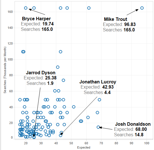
Similarly, we can break down each player’s xR₄ by the value produced on each type of batted ball. Here are graphs for xR₄ produced on each of the four types of batted balls resulting from a swing, with respect to the number of batted balls of that type hit by the player. For simplicity, from this point on, when I drop the subscript when describing a batter’s expected run total, I’m referring to xR₄.

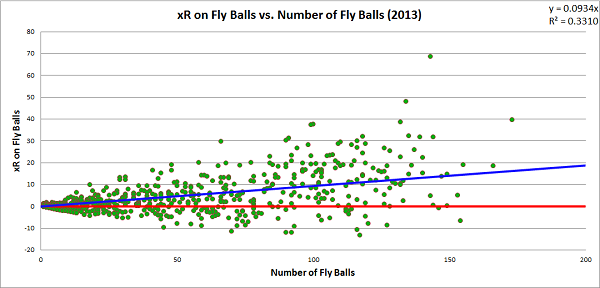
Line drives are the most optimal result for a batter. The first objective of batters is to reach base safely, and they did that on 67.0 percent of line drives last season. No batter who hit at least eight line drives in 2013 caused a net decrease in his team’s run expectancy during those events. For most batters, hitting the ball into the outfield in the air is the ideal way to produce value, as fly ball production tends to create a positive change in a team’s run expectancy. However, fly balls have the most variance of any of the batted ball types, and there are certainly batters who hurt their teams more when hitting the ball at a high launch angle than a low one. Here are the players to produce the lowest xRA on fly balls last season (minimum 50 fly balls):

For each of these batters, hitting the ball on the ground or on a line drive were far better results on average.

While groundballs may be a preferable result for some batters when compared to fly balls, they are still effectively batting failures for the team. There were 840 batters in 2013 to hit at least one groundball and only 44 produced a net positive change in their team’s run expectancy. Of those 44 players, only 11 hit more than 10 groundballs, and only two (Mike Trout and Juan Francisco) hit at least 100 groundballs. Here are the players with the highest xRA on groundballs in 2013 who hit at least 100 groundballs:

xR₄ allows us to tell the most detailed story concerning the type of value a batter produced, independent of the situational context at the time the plate appearance occurred. Because we gradually added layers of detail to our estimation, we can compare how each level of expected runs correlates to this most detailed level. In this way, we can judge how much information each level provides with respect to our most detailed estimation. Here is a graph that charts a batter’s xR₄ with respect to his xR₁, xR₂, and xR₃ estimations:

The line that cuts through the data reflects the xR₄ values charted against themselves. For each xR_n, we can calculate how well it correlates with xR₄ and, consequently, how much of xR₄ it can explain. Remember that we have already shown that xR₁ has a direct linear correlation with eOBA and xR₂ has a very high, though not quite direct, correlation with eTBA. For the xR₁ values, we observe a correlation, r, with xR₄ of .912, and an r² of .832, meaning that knowing the rate at which a batter reaches base explains over four-fifths of our estimation of xR₄. For the xR₂ values, r² increases to .986; for the xR₃ values, r² increases slightly higher to .990.[iv]

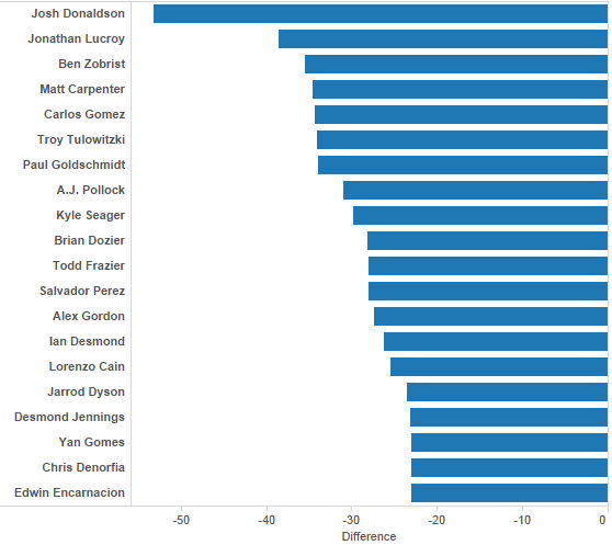
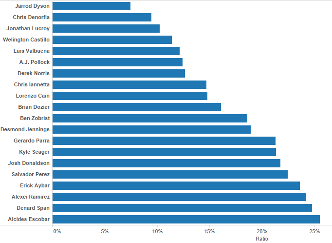
The takeaway from this is that when considering the whole population of players, there is little difference in a run estimator that considers the batted-ball context and one that does not; you can still explain 99 percent of the value estimated by xR₄ by stopping at xR₃. In fact, if all you know is the rate at which a batter accomplishes his two main objectives—reaching base and advancing as far as possible—you can explain well over 90 percent of the value estimated by xR₄. However, on an individual level, there is enough variation that observing the batted-ball context can be beneficial. Here are the five players with the largest positive and negative differences between their xR₃ and xR₄ estimations:

These changes are not massive, and these are the extreme cases for 2013, but they are certainly large enough that ignoring them will weaken specific analyses of batting production. Incorporating batted ball details into our analysis adds a significant layer of complexity to our calculation, but it must be considered if we want to tell the most accurate story of the value a batter produced.

If this work seems at all familiar, you may have read this article that I wrote last year on a statistic that I called Offensive Value Added (OVA). For all intents and purposes, OVA and xR are identical. I decided that the name change to xR would help me differentiate estimations more simply, as I could avoid naming four separate statistics for each level of contextual detail, but there was also a secondary reason for changing the presentation of the data. OVAr was the rate statistic associated with OVA, and it was scaled to look like a batting average, much in the same way that wOBA is scaled to look like an on base average. At the time, I choose to do this to make it easier to appreciate how a batter performed, since many baseball enthusiasts are comfortable interpreting the relative significant of a batting average.

After thinking on the subject, though, I came to decide that I prefer statistics that actually “mean” something to those that give a general, unit-less rating. For instance, try to explain what wOBA actually reflects. It starts as a run estimator, but then it’s transformed into a number that looks like a statistic with specific units (OBA), while not actually using those units. Once that transformation occurs, it no longer reflects anything specific and only serves as a way to rate batters. The same principle applies to other statistics as well, most notably OPS, which is arguably the most meaningless of all baseball statistics, perhaps all statistics ever (don’t get me started).

xR and xRA estimate the change in a team’s run expectancy caused by a batter’s plate appearances. They are measured in runs and runs per plate appearance, respectively. xRA may not look like a number you’ve seen before, and generally needs to be written out to four decimal places instead of three, unlike basic averages, but it’s linguistically very simple to use and understand. I’d rather sacrifice the comfort of having a statistic merely look familiar and instead have it actually reflect something tangible. This doesn’t take away from the value of a statistic like wOBA, which is a great run estimator no matter what scale it is on; a lack of meaning certainly does not imply a lack of value. Introducing an unscaled run average, xRA, will hopefully create a different perspective on how to talk about batting production.

There is one final expected run estimation that I want to consider that could easily cover an entire new part on its own, but I’ll limit myself to just a few paragraphs. The xR estimations we have built have been constructed independent of the situational context at the time of the batter’s plate appearance. Since we want to cover the entire spectrum of context-neutral run estimation to context-specific run estimation, we will conclude by considering xR_s, which is an estimate of the change in a team’s run expectancy based on the out/base state before and after the action of the plate appearance. This is very nearly the same thing as RE24 but it only considers runs produced due to the primary action of plate appearances and not baserunning events.

In many respects, xR_s is the simplest run estimator to construct of all that we have built thus far. There are only three pieces of information you need to know in a given plate appearance to construct xR_s: the run-scoring environment, the out/base state at the start of the action of the plate appearance, and the out/base state at the end of the action of the plate appearance. Next time you go to a baseball game, bring along a copy of a run expectancy matrix, like the one provided earlier. On a scorecard, at the start of every plate appearance, take note of the value assigned to the out/base state, making adjustments if any runners move while the batter is still in the batter’s box. Once the plate appearance is over, note the value of the new out/base state, separating out any advancement on secondary fielding errors or throws to other bases. Subtract the first value from the second value, and add in any RBIs on the play, and write the number in the box associated with the batter’s plate appearance; you just calculated xR_s. Do this for a whole game, and you will have a picture of the total value produced by every batter based on the out/base state context in which they performed.

The effective averages and expected run estimations provide a foundation on which batting analysis can be performed. They combine both “real and indisputable facts” with detailed estimations of the run produced in every event in which a batter participates. Any story that aims to describe the value that a batter provides to his team must consider these statistics, as they are the only ones which account for all value produced. 147 years ago, Henry Chadwick suggested that batters should be judged on whether they passed a “test of skill.” I think they should be judged on whether they passed a “test of value.”

Thanks to Benjamin H Byron for editorial assistance, as well as the staff at the Library of Congress for assistance in locating original copies of the 19^th century newspaper articles included in Part 1.

Here is data on eOBA, eTBA, and each level of xR and xRA estimation, for each batter in 2013.

Bibliography

[i] I’ll be focusing on 2013 because the full season is complete. All the work described here could easily be applied to 2014, or any other season, I just don’t want to use incomplete information.

[ii] While these terms are used a lot, there aren’t any specific definitions commonly accepted that differentiate each type of batted ball. For terms used so commonly, it doesn’t make much sense to me that they are not well defined. It won’t apply to the data used in this research, but here is my attempt at defining them.

A bunt is a batted ball not swung at but intentionally met with the bat. A groundball is a batted ball swung at that lands anywhere between home plate and the outer edge of the infield dirt and would be classified as a line drive if it made contact with a fielder in the air. A line drive is a batted ball swung at that leaves the bat at an angle of at most 20° above parallel to the ground (the launch angle), and either lands in the outfield or makes contact with any fielder before landing (generally through a catch, but sometimes a deflection). A fly ball is a batted ball swung at, with a launch angle between 20° and 60° above parallel (not inclusive), that either lands in the outfield or is caught in the air by a player in the outfield. A popup is a batted ball swung at that either (a) leaves the bat at an angle of 60° or greater above parallel and lands or is caught in the air in the outfield, or (b) leaves the bat at an angle greater than 30° and lands or is caught in the air in the  infield.

This would result in some balls being classified differently than they currently are, and not just because differentiating between a line drive and a fly ball is somewhat difficult with just a pair of eyes. If the defense were to play an infield shift, and the batter were to hit a line drive into the outfield grass into that shift, subsequently being thrown out at first base, it would likely be called a groundout by current standards. Batted balls should not be defined based on defensive success or failure, but by the general path which they take when leaving the bat. It may be unusual to credit a batter with making a line out despite the ball hitting the ground, but it more accurately reflects the type of ball put into play by the batter.

I don’t know that these are the “correct” ways to group together these events, but as we now are using technology that tracks the flight of the baseball from the moment it is released by the pitcher through the end of the play, we should probably have better definitions for types of batted balls than those currently provided by MLB. I don’t expect a human stringer to be able to differentiate between a ball hit with a 15° launch angle or a 25° launch angle, but that doesn’t mean we shouldn’t have some standard definition for which they should aim.

[iii] In theory, xR₅ would attempt to consider details that are even more specific, perhaps the initial velocity of the ball off the bat, the launch angle, and whatever other information can be gleaned from technology like HIT F/X. The xR framework leaves room to consider any further amount of detail that a researcher wants to consider.

[iv] Though not charted here, the r² value based on the correlation between wRAA, the “counting” version of wOBA, and xR₄ is .984. As wRAA is nearly identical to xR₃ but excludes a few of the more rare events from its calculation, it’s not surprising that the r² value between wRAA and xR₄ is just slightly smaller than the r² between xR₃ and xR₄.

Dear FanGraphs community,

This isn’t a post about baseball, per se, but rather about the way we talk about it. Lately, I’ve been thinking a lot about how to improve the quality of dialogue surrounding sabermetrics. Please excuse my rambling, as I tend to get rather emotional and philosophical when discussing this particular topic.

When reading posts and especially comments, I sometimes get the sense that we think we are right merely due to the fact that statistics are objective. In a sense, this is true. As long as the methodology is clearly laid out, stats really are just numbers. But people are biased. All language is persuasive in some sense, and the inherent neutrality of numbers is often hijacked by various human agendas. Sabermetrics are not exempt from this phenomenon.

Most modern discourse surrounding baseball analysis pits “old-school” vs. “new-school” in a largely arbitrary ideological cage fight. These sorts of polemical constructs make for good television, but slow progress. Its easy to get caught up in the excitement of a debate while completely missing out on what really matters. Baseball is a beautiful game and it brings people together. It’s America’s pastime for a reason! It transcends cultural differences, generation gaps, and even language itself.

Statistics help us to understand and evaluate how well this great game is being played. They act as a mental “handle” by which we can intellectually grasp the importance of each individual event and performance. Everyone, regardless of their stance on sabermetrics, wants statistics that are both intuitive and accurate. So let’s set aside our agendas for a minute and think about how to proactively bridge the gap between these two sides that have so much to offer!

For starters, we should minimize our implementation of hostile methodologies. Getting on a soapbox and proclaiming the evils of traditionalism simply doesn’t do anybody any good. It feeds our pride, as well as the opposition’s presumption that we care more about our statistics than we do about, you know, actual baseball. Over the last few years, I’ve begun to think of myself more as a teacher of sabermetrics than a defender of them. This approach has two important ramifications.

First, it dictates that we get along with those who disagree with us. In my experience, people are only open to new information in the context of a trusting relationship. As fellow baseball fanatics, we have an easy point of contact with traditionalists: we both like baseball. Duh! Focus on that first rather than stuffing a lecture on DIPS theory down their throats.

Second, a teaching disposition encourages us to refine and adapt our communication of sabermetric concepts. Next time you want to call someone a nincompoop on a message board, first ask yourself, “What could I have done to explain this idea more clearly.” Chances are, the person isn’t stupid, just unenlightened and/or overly argumentative. Over my next few posts, I’ll get into the nitty-gritty of how we might make this happen.

Contrary to popular belief, numbers aren’t evil. Baseball statistics in particular have come a long way toward being less deceptive. Let’s represent them well, shall we?

Sincerely yours,

KK-Swizzle

Lists of baseball’s most underrated players are often interesting and thought-provoking exercises, because by definition they focus on players that tend to get less attention than they should. However, there isn’t an easy way to definitively say how players are “rated” by baseball followers. Writers often just list off players who have the attributes that they are looking for (grit, plate discipline, small market players, etc.), which isn’t a bad way of doing it.

However, there is a more scientific way of approaching a list like this. We could look at how many people are doing Google searches for specific players. It wouldn’t exactly tell us what players are most underrated, but it can tell us which players should be getting more attention; these two things are very tightly correlated. The key difference is that plenty of players get attention for things that don’t necessarily mean they are considered good players. Ryan Braun got a lot of attention during his steroid drama, Robinson Cano was heavily talked about during free agency, and people search for Carlos Santana because of this and this. But when good players draw very little interest from fans, they’re probably underrated. But the term I’ll use is under-popular.

Using Google’s Adwords Keyword Tool, I gathered the data on every player who has achieved a WAR of at least 3.0 since the beginning of the 2013 season. A regression model with those 132 players showed that an additional 1 WAR was worth 6,000 Google searches per month – not too shabby.

Here is a plot of these players, with the expected amount of Google searches on the horizontal axis, and the actual amount of searches on the vertical. While the keyword tool was incredibly useful, it rounds numbers when they get too high, and you can see a handful of players were rounded off to exactly 165,000 searches per month (FYI, these players were Mike Trout, Miguel Cabrera, David Ortiz, Robinson Cano, Bryce Harper, and Yasiel Puig). Derek Jeter has roughly double that amount, but his WAR did not qualify him for this list.

There are a lot of players who have played very well the last two years who are by no means household names. Welington Castillo has put up 3.8 WAR since the start of 2013, A.J. Pollock has been worth 6.1 wins, and Brian Dozier 5.8. In order to really measure who the most under-popular players are, I’ll use two methods. The first is just to simply subtract how many Google searches were expected and how many there really were.

According to this measurement, Josh Donaldson is the most under-popular player in baseball, because he should have been looked up 53,000 times per month more often than he was (68k vs. 15k). That’s a big difference. There are some excellent players on this list, with many players who have an argument as the best or one of the few best players at their position. But for the most part, these are well known players who should just be more well known.

A different way to measure under-popularity, and the way I think is more telling, is to find the ratio between expected and actual searches, as opposed to just subtracting. For instance, is Edwin Encarnacion more under-popular than, say, Luis Valbuena? Encarnacion should have gotten 41,000 searches per month, but actually only got 18,000. Valbuena, however, played like someone who should have been searched 20,000 times, but was only Googled 2,400 per month. Since I believe Valbuena’s numbers are more out of whack, I prefer the second method.

Here are the top 20 players using that measurement, where we see how many times a player was searched as a percentage of how many times you would expect them to be:

Jarrod Dyson has quietly become a well above average baseball player. In about 800 career PA, Dyson has a WAR of 6.8. That is All-Star level production. His elite fielding and baserunning skills (which have combined to be worth more than 3 wins these last two years) make his wRC+ of 91 more than acceptable.

A.J. Pollock appears high on both lists, and for great reason. This year he is quietly hitting .316/.366/.554, after putting up 3.6 WAR last year.

This method of establishing players who deserve more credit for their play certainly has some flaws. WAR is not the only way to measure how good a player is, and Google searches are not a perfect representation of how popular or famous players are. However, it takes away the guess work and opinions from the standard underrated player lists, and in that there is some value.

I. Introduction

In the statistics driven sport of baseball, the fans who once enjoyed recording each game in their scorecard have become less accepting of what they observe and now seek to validate each observation with statistics.  If the current statistics cannot support these observations, then they will seek new and authenticated statistics.

The following sections contain formulas for statistics I have not encountered, yet piqued my curiosity, regarding the 2010 Giants’ World Series starting rotation.  Built around Tim Lincecum, Matt Cain, Jonathan Sanchez, and Madison Bumgarner, the 2010 Giants’ strength was indeed starting pitching.  Each player was picked from the Giants farm system, three of them would throw a no-hitter (or perfecto) as a Giant, and of course they were the 2010 World Series champions.  Throw in a pair of Cy Young awards (Lincecum), another championship two years later (Cain, Bumgarner, Lincecum), eight all-star appearances between them (Cain, Bumgarner, Lincecum), and this rotation is highly decorated.  But were they an elite rotation?

II. Perfectos & No-No’s

It certainly seems rare to have a trio of no-hit pitchers on the same team, let alone home-grown and on the same championship team.  No-hitters and perfect games factor in the tangible (a pitcher’s ability to get a batter out and the range of the defense behind him) and the intangible (the fortitude to not buckle with each accumulated out).  Tim Lincecum, Matt Cain, and Jonathan Sanchez each accomplished this feat before reaching 217th career starts, but how many starts would we have expected from each pitcher to throw a no-hitter or perfect game?  What is the probability of a no-hitter or perfect game for each pitcher?  We definitely need to savor these rare feats.  Based on the history of starting pitchers with career multiple no-hitters, it is unlikely that any of them will throw a no-hitter or perfect game again.  Nevermind, it happened again for Lincecum a few days ago.

First we deduce the probability of a perfect game from the probability of 27 consecutive outs:

Table 2.1: Perfect Game Probabilities by Pitcher

The probability of a perfect game is calculated for each pitcher (above) using their exact career on-base percentage (OBP rounded to three digits) through the 2013 season.  Based on these calculations, we would expect 1 in 12,152 of Matt Cains starts to be perfect.  Although it didn’t take 12,152 starts to reach this plateau, he achieved his perfecto by his 216th start.  For Tim Lincecum, we would expect 1 in 19,622 starts to be perfect; but starting even 800 starts in a career is very farfetched.   Durable pitchers like Roger Clemens and Greg Maddux only started as many as 707 and 740 games respectively in their careers and neither threw a perfect game nor a no-hitter.  No matter how elite or if Hall of Fame bound, throwing a perfect game for any starting pitcher is very unlikely and never guaranteed.  However, that infinitesimal chance does exist.  The probability that Jonathan Sanchez would throw a perfect game is a barely existent chance of 1 in 94,488, but he was one error away from a throwing a perfect game during his no-hitter.

The structure of a no-hitter is very similar to a perfect game with the requirement of 27 outs, but we include the possibility of bb walks and hbp hit-by-pitches (where bb+hbp≥1) randomly interspersed between these outs (with the 27th out the last occurrence of the game).  We exclude the chance of an error because it is not directly attributed to any ability of the pitcher.  In total, a starting pitcher will face 27+bb+hbp batters in a no-hitter.  Using these guidelines, the probability of a no-hitter can be constructed into a calculable formula based on a starting pitcher’s on-base percentage, the probability of a walk, and the probability of a hit-by-pitch.  Later we will see that this probability can be reduced into a simpler and more intuitive formula.

Let h, bb, hbp be random variables for hits, walks, and hit-by-pitches and let P(H), P(BB), P(HBP) be their respective probabilities for a specific starting pitcher, such that OBP = P(H) + P(BB) + P(HBP).  The probability of a no-hitter or perfect game for a specific pitcher can be constructed from the following negative multinomial distribution (with proof included):

This formula easily reduces to the probability of a no-hitter by subtracting the probability of a perfect game:

The no-hitter probability may not be immediately intuitive, but we just need to make sense of the derived formula. Let’s first deconstruct what we do know… The no-hitter or perfect game probability is built from 27 consecutive “events” similar to how the perfect game probability is built from 27 consecutive outs.  These “event” and out probabilities can both broken down into a more rudimentary formulas. The out probability has the following basic derivation:

The “event” probability shares a comparable derivation that utilizes the derived out probability and the assumption that sacrifice flies are usually negligible per starting pitcher per season:

From this breakdown it becomes clear that the no-hitter (or perfect game) probability is logically constructed from 27 consecutive at bats that do not result in a hit, whose frequency we can calculate by using the batting average (BA). Recall that a walk, hit-by-pitch, or sacrifice fly does not count as an at bat, so we only need to account for hits in the no-hitter or perfect game probability. Hence, the batting average in conjunction with the on-base percentage, which does include walks and hit-by-pitches, will provide an accurate approximation of our original no-hitter probability:

Comparing the approximate no-hitter probabilities to their respective exact no-hitter probabilities in Table 2.2, we see that these approximations are indeed in the same ball park as their exact counterparts.

Table 2.2: No-Hitter Probabilities by Pitcher

The probability of a no-hitter is calculated for each pitcher (above) using their exact career on-base percentage, walk probability, and hit-by-pitch probability through the 2013 season.  Notice that the likelihood of throwing a no-no is significantly greater than that of a perfecto for each pitcher.  For example, Lincecum and Cain’s chances of making no-no history are far easier than being perfect by the respective factors of 15.9 and 11.5.  Although Lincecum and Cain are still both unlikely to accumulate the 1,231 and 1,055 starts necessary to ascertain these no-hitter probabilities.  If it’s any consolation, Lincecum already achieved his no-hitter by his 207th start (and another by his 236th start) and Cain already has a perfecto instead.

Furthermore, it’s possible for two pitchers with disparate perfect game probabilities to have very similar no-hitter probabilities, as we see with Sanchez and Bumgarner.  Sanchez has a no-hitter probability of 1 in 1,681 that is 56.2 times greater than his perfect game probability, while Bumgarner’s 1 in 1,772 probability is a mere 6.1 times greater.  This discrepancy can be attributed to Sanchez’ improved ability to not induce hits versus his tendency to walk batters, while Bumgarner’s improvement is of a lesser degree.  Regardless, Sanchez’ early no-hitter, achieved by his 54th start, can instill hope in Bumgarner to also beat the odds and join his 2010 rotation mates in the perfect game or no-hitter’s club.  Adding Bumgarner to the brotherhood would greatly support the claim that the Giants 2010 starting rotation was extraordinary.  However, the odds still fall in my favor that I will not need to rewrite this section of this study due to another unexpected no-no or perfecto by Lincecum, Cain, Sanchez, or Bumgarner.

Let’s face it: we’re all nerds here at FanGraphs. But it takes a special kind of nerd to bring FanGraphs’ brand of sabermetric analysis to that other realm of the dull and dweeby: the United States Congress.

Every summer, a handful of the 535 senators and congressmen who represent you in Washington divide into teams to play the Congressional Baseball Game, a charity event at Nationals Park. Despite its informal nature and the, ah, senescent quality of play, the game is a serious affair (something its participants often have experience with). This is no friendly softball game; the teams practice for months before the big day, and the players take the results very seriously.

So seriously, in fact, that players keep track of (even send press releases about) their hits and RBI. A small group of baseball-obsessed politicos scores and generates a box score for the game every year. With their help, I was able to take their record-keeping to the next level. This is where this becomes the dorkiest FanGraphs article ever—for the first time, we now have advanced metrics on the performance and value of U.S. congressmen’s baseball skills.

Using recent Congressional Baseball Game scoresheets, I made a Google spreadsheet that should look familiar to any FanGraphs user—complete with the full Standard, Advanced, and Value sections you see on every player page. (Though this spreadsheet is more akin to the leaderboards—since the game is only played once a year, I treated the entire, decades-long series as one “season,” and each line is a player’s career stats in the CBG.) From Rand Paul’s wOBA to Joe Baca’s FIP-, all stats are defined as they are in the Library and calculated as FanGraphs does for real MLBers—making this the definitive source for the small but vocal SABR-cum-CBG community.

That said, unfortunately the metrics can never be complete—there’s just too much data we don’t have. Most notably, although the CBG has a long history (dating back to 1909), I capped myself at stats from the past four years only—so standard small-sample-size caveats apply. (This is mostly for fun, anyway.) Batted-ball data is also incomplete, so I opted to leave it out entirely—and we don’t have enough information about the context of each at-bat to calculate win probabilities. For obvious reasons, there’s also no PITCHf/x data, and fielding stats are a rabbit hole I’m not even going to try to go down.

It’s still a good deal of info, though, and there’s plenty to pick through that goes beyond what you might have noticed with the naked eye at the past four Congressional Baseball Games. But why should I care to pick through them, you might ask; what good are sabermetrics for a friendly game between middle-aged men? Well, apart from the always-fun Hall of Fame arguments, they serve the same purpose they do in the majors: they help us understand the game, and they can help us predict who will win when the Democrats next meet the Republicans (how else would the teams be divided?) on the battle diamond—this Wednesday, June 25.

You probably don’t need advanced metrics to guess that the Democrats are favored. They’ve won the past five games in a row, including the four in our spreadsheet by a combined score of 61 to 12. That’s going to skew our data, but by the same token, Democratic players have clearly been better in recent years. Going by WAR, a full five Democrats are better than the best Republican player, John Shimkus of Illinois.

But the reason we expect Democrats to win on Wednesday is the player who tops that list: Congressman Cedric Richmond of Louisiana. Richmond’s 1.1 WAR (in only three games!) is 0.9 higher than the next-best player (Colorado’s Jared Polis), putting him in a league of his own. In each of the past three CBGs, the former Morehouse College varsity ballplayer has pitched complete-game gems that have stifled the Republican offense. He carries a 40.0% K% and 28 ERA- into this year’s game. (Note: Congressional Baseball Games last only seven innings, so the appropriate pitching stats use 7 as their innings/game constant in place of MLB’s 9.)

The GOP has a few options to oppose Richmond on the mound—it’s just that none of them are good. The four Republicans on the roster with pitching experience have past ERAs ranging from 8.08 to 15.75. If there’s any silver lining, it’s that Republican pitchers have been somewhat unlucky. Marlin Stutzman has a .500 BABIP, and Shimkus has an improbably low 20.8% LOB percentage. Thanks to a solid 15.0% K-BB%, Stutzman has just a 5.98 FIP—high by major-league standards, but actually exactly average (a FIP- of 100) in the high-scoring environment of the CBG. (Another note: xFIP is useless in the congressional baseball world, as no one has hit an outside-the-park home run since 1997.) A piece of advice to GOP manager Joe Barton of Texas: Stutzman is your best option for limiting the damage on Wednesday.

On offense, it’s again the Cedric Richmond show. His 8 wRC and 4.6 wRAA dwarf all other players. In a league where power is almost nonexistent, he carries a .364 ISO (his full batting line is a fun .818/.833/1.182); only eight other active players even have an ISO higher than .000. Other offensive standouts for the Democrats include Florida’s Patrick Murphy, he of the 214 wRC+ and .708 wOBA (using 2012 coefficients), and Missouri’s Lacy Clay, who excels on the basepaths to the tune of a league-high 0.5 wSB. With a 1.4 RAR (fourth-best in the league) despite only two career plate appearances, Clay has proven to be the best of the CBG’s many designated pinch-runners who proliferate in the later innings. (Caveat: UBR is another of those statistics we just don’t have enough information to calculate.) Democrats might want to consider starting him over Connecticut Senator Chris Murphy, however; Murphy is a fixture at catcher for the blue team despite a career .080 wOBA and -2.5 wRAA.

As on the mound, Republicans don’t have a lot of talent at the plate. Their best hitter is probably new Majority Whip Steve Scalise, who has a 168 wRC+, albeit in just four plate appearances. (Scouting reports actually indicate that Florida Rep. Ron DeSantis is actually their best player, but injury problems have kept him from making an in-game impact so far in his career—and he’s missing this game entirely due to a shoulder injury.) Meanwhile, uninspired performers like Jeff Flake (.268 wOBA) and Kevin Brady (.263 wOBA) continue to anchor the GOP lineup, potentially (rightfully?) putting their manager on the hot seat. Some free advice for the Republicans: try to work the walk better. Low OBPs are an issue up and down the lineup, and they have a .279 OBP as a team. Their team walk rate of 8.2% is also too low for what is essentially a glorified beer league. If someone is telling them that the way to succeed against a pitcher of Richmond’s caliber is to be aggressive, they should look at the numbers and rethink.

There are many arguments against the sacrifice bunt, by many sabermetricians and sports writers, all with the purpose of retiring its practice in baseball. The three main reasons not to bunt are that it gives away an out (out of only 27), the rate of scoring goes down (based on ERT by Tango), and that most bunters are unsuccessful.

For my argument, I will establish a more romantic approach and one I haven’t seen across the world of sabermetrics. With this approach, I will land on a conclusion that supports the sacrifice bunt and even speaks to the expansion of its practice.

Bunters can be successful

First, I’ll attack the last argument. If bunting is coached, bunters will be better. In my own research, as well as research done by others, I’ve found that there have been years when even the pitchers are able to bunt successfully over 90% of the time. Many people say that practice makes perfect, and while perfection might not be reached in the batters box, I wouldn’t be surprised if bunters were allowed to get close, or at least to their abilities in the 80’s.

Innings are more prosperous after bunt

The second argument is the main staple of this essay. In the world of analytics, general numbers are not good enough to explain why a phenomena is bad. Tom Tango’s famous Run Expectancy Matrix is used to make arguments against bunting across the Internet. Unfortunately, it’s assumed that the situations just exist rather than being set up the way that they are. It would be appropriate to use the table if a team were allowed to place a man, or men, on a base, or bases, and set the number of outs. However, as a strong believer in the principle of sufficient reason, I believe that there’s variability between a man on second with one out from a bunt and a man on second with one out from other situations.

For this reason, I set up my own analysis through the resource of Retrosheet play by play for the years of 2010-2013. To make things simple and not delve too deeply in varying circumstances, I will simply use larger data sets and noticeable differences to tell a story. First, I will look at only innings that start with men on base before the first out. Sacrifice bunts cannot happen when men are not on base, so it would be unfair to statistically compare innings with bunts to just innings without bunts. In line with Retrosheet’s system, I’m looking at all instances of SH, when they occur before (and usually result in) the first out.

To summarize, I’ll be looking at the percent chance that a team scores in an inning where they are able to get a man, or men, on base before the first out (as well as the average runs per inning when that situation is set up). I will compare this base situation to the percent chance that a team scores in an inning when they decide to sacrifice for that first out (as well as the average runs per inning when that situation is set up).

This data can be seen below with a total of about 53,000 innings across seasons where men were on base before the first out. In general, through the four years, teams score in about 26.8% of innings with about 0.478 runs per inning (RPI); when men get on base before the first out, they score 45.8% of innings with a .691 RPI. (In innings where a leadoff HR is hit, this does not count as men on base (nor will these runs count in calculation of either group, assuming men get on after the home run is hit, and before an out)).

Many managers, if not statisticians, understand this increase in the chance to score a run; after all, that’s why they do it. In 2010 and 2013, deciding to, and successfully laying down a sacrifice bunt resulted in a 13% increase in the ability to score that inning for the AL. And while it would make sense that the argument stops there, RPI also supports the sacrifice bunt (with data of the last four years). (Here, again, RPI = Runs scored after MOB B1O situation divided by number of innings of situation.)

This increase in RPI (seen as high as 0.137 Runs Per Inning larger than without bunting, 2012 AL) can contribute a decent number of runs over the course of a season. For example, in 2013, if the Oakland Athletics bunted a little less than once per series, they would have been on par with National League teams with number of bunts (in the 60’s). If they were able to bunt 47 more times (68, rather than 21), then their run total would have given them enough wins to have the best record in baseball (using Bill James adjusted pythagorean expected win percentage).

To summarize, an adjusted estimated runs table with respect to sacrifice bunt set up positioning and outs would produce more runs than the average table that does not take into concern how outs or players arrived at their position. This argument was suggested at the end of an essay by Dan Levitt, with earlier data in a more complex and subtle manner. RPI and the probability of scoring a run increase with a sacrifice bunt.

Bunting is symbolic of the greater good

The first and final argument to discuss is the idea that a sacrifice bunt throws away an out. In baseball, if a player bats out of order, or does not run out an error (among other mental mistakes), then that is giving away an out. And I believe that if a coach tells a player that he can’t hit, and to bunt because he can’t hit, then I wouldn’t argue that in those cases, you are giving away an out (knowingly removing the opportunity from the player to get a hit). So unless you believe that’s how coaches interact with their players prior to calling for the bunt, I will disagree with that notion.

The dictionary definition of sacrifice is “an act of giving up something valued for the sake of something else regarded as more important or worthy.” It’s the biggest theme in religious studies, the coolest way to die in movies, and the plot for heroic stories in the nightly news. Eliminating the psychological effects of a sacrifice, where they’re common place in our culture, seems slightly irresponsible after seeing the data.

This idea lends nicely to the discrepancy between American and National Leagues. Articles can be found, research has been done, and the common thought among those surrounding the game is that pitchers should bunt because they won’t do much else (in appropriate situations). In fact, an article by James Click gives the opinion that the lower the average, the more advantageous it is to bunt. However, my argument is the opposite. The amount they sacrifice, if they’re unable to hit is not valuable to those involved. If the pitcher is respected as a hitter, then their sacrifice is meaningful. Mentally as a leadoff man, if your pitcher is hitting sub .100, and there’s a man on base, he’s bunting because he cannot hit. That’s not a teamwork inspired motive, that’s a picking poison motive. The chart below shows data from the last four years when men get on base before the first out, it distinguishes that the National League is better than either league that doesn’t bunt, but far from as effective as AL bunters.

The argument can be made that the AL contains better hitters, and while I believe this, there would be a larger separation of the % scoring without bunting as well as the RPI of the innings where players get on before the first out.

Because of this separation, I feel that bunting is not giving away an out, but sacrificing for something greater. Simply put, if my teammate sets me up to knock in a run with a hit, that’s easier that having to find a gap, or doing something greater. In many cases, I might need to just find a hole in the infield. Also, I know that my team, and coach, believes in me to be successful. Professional athletes can’t possibly feel pressure and confidence that emanates from teammates with the hopes of greater success, that idea would be ridiculous, right? Those ideas are practiced and taught in business places and self-help books around the world.

Opposition

The data that I used was from Retrosheet, and while this data lists a lot of SH’s (sacrifice bunts) from where errors occur, to double plays, the main output is the standard sacrifice bunt. That being said, it does not include instances where the batter was bunting for a base hit (regardless of number of men on base), or other strange incidents of sacrifice failures (places where the scoring did not distinguish that an SH was in play). After recreating the analysis to include all bunts, the values of RPI and % scoring assuming men on base before the first out, values were still larger than without the bunt, but not as large as the sacrifice representation. This argument falls with the established idea that bunting could be more successful than most people think (especially when the bunt is a sacrifice). For instance, if the numbers above are reduced by as much as 85% in some cases, it still produces more successful results.

The next piece of opposition is that different circumstances have different weights in these situations, and that my case is too general to provide an advantage to a staff trying to decide whether to bunt. My argument is that upon analyzing circumstances, the most important element is the sacrifice bunt. In most situations, I feel that it will boost the team’s ability (and desire) to have success. With four years of data, my goal was to be able to refute the reliance on the simple Tango Run Expectancy Matrix, and how it is used, not to recreate one. In my opinion, in order for people to understand how historically successful situations have been, there should be hundreds of Run Expectancy Matrices highlighting how runners came to be where they are, as well as what batters follow.

The final piece of opposition has been created by myself during the generation of this essay or idea. The Heisenberg Uncertainty Principle relates to the ability to study the speed and position of a microscopic particle. Simply put, by studying one, you’re unable to observe the other. The act of observation limits the ability to fully observe. Because my argument is set up in a romantic sense, it could be argued that this principle relates. If coaches and teams start bunting every other inning, the act of giving oneself away for the greater good of the team will diminish and its advantage psychologically will wither away. In other words, the knowledge of how something effects one emotionally can limit one from being emotionally affected. I present this as an opposition because I feel that this might already be the case where if a pitcher is repeatedly bunting, teams will not think much of it as a quest for the greater good. However, when players are seen as an asset in the box, this advantage still exists; so teammates can still be sold on the relevance of the opportunity.

If these ideas spread, will this essay result in more bunts, especially when there are no outs? Probably not, because statisticians are stubborn. But it definitely provides an outlet for coaches who support the old school, traditional game of baseball.

I’ve decided to break this final section in half and address the early development of run estimation statistics first, and then examine new ways to make these estimations next week. In Part 1, we examined the early development of batting statistics. In Part 2, we broke down the weaknesses of these statistics and introduced new averages based on “real and indisputable facts.” In Part 3, we will examine methods used to estimate the value of batting events in terms of their fundamental purpose: run creation.

The two main objectives of batters are to not cause an out and to advance as many bases as possible. These objectives exist as a way for batters to accomplish the most fundamental purpose of all players on offense: to create runs. The basic effective averages presented in Part 2 provide a simple way to observe the rate at which batters succeed at their main objectives, but they do not inform us on how those successes lead to the creation of runs. To gather this information, we’ll apply a method of estimating the run values of events that can trace its roots back nearly a century.

The earliest attempt to estimate the run value of batting events came in the March 1916 issue of Baseball Magazine. F.C. Lane, editor of the magazine, discussed the weakness of batting average as a measure of batting effectiveness in an article titled “Why the System of Batting Averages Should be Changed”:

“The system of keeping batting averages…gives the comparative number of times a player makes a hit without paying any attention to the importance of that hit. Home runs and scratch singles are all bulged together on the same footing, when everybody knows that one is vastly more important than the other.”

To address this issue, Lane considered the fundamental purpose of making hits.

“Hits are not made as mere spectacular displays of batting ability; they are made for a purpose, namely, to assist in the all-important labor of scoring runs. Their entire value lies in their value as run producers.”

In order to measure the “comparative ability” of batters, Lane suggests a general rule for evaluating hits:

“It would be grossly inaccurate to claim that a hit should be rated in value solely upon its direct and immediate effect in producing runs. The only rule to be applied is the average value of a hit in terms of runs produced under average conditions throughout a season.”

He then proposed a method to estimate the value of each type of hit based on the number of bases that the batter and all baserunners advanced on average during each type of hit. Lane’s premise was that each base was worth one-fourth of a run, as it takes the advancement through four bases for a player to secure a run. By accounting for all of the bases advanced by a batter and the baserunners due to a hit, he could determine the number of runs that the hit created. However, as the data necessary to actually implement this method did not exist in March 1916, the work done in this article was little more than a back-of-the-envelope calculation built on assumptions concerning how often baserunners were on base during hits and how far they tended to advance because of those hits.

As he wanted to conduct a rigorous analysis with this method, Lane spent the summer of 1916 compiling data on 1,000 hits from “a little over sixty-two games”[i] to aid him in this work. During these games, he would note “how far the man making the hit advanced, whether or not he scored, and also how far he advanced other runners, if any, who were occupying the bases at the time.” Additionally, in any instance when a batter who had made a hit was removed from the base paths due to a subsequent fielder’s choice, he would note how far the replacement baserunner advanced.

Lane presented this data in the January 1917 issue of Baseball Magazine in an article titled similarly to his earlier work: “Why the System of Batting Averages Should be Reformed.” Using the collected data, Lane developed two methods for estimating the run value that each type of hit provided for a team on average. The first method, the one he initially presented in March 1916, which I’ll call the “advancement” method,[ii] counted the total number of bases that the batter and the baserunners advanced during a hit, and any bases that were advanced to by batters on a fielder’s choice following a hit (an addition not included in the first article). For example, of the 1,000 hits Lane observed, 789 were singles. Those singles resulted in the batter advancing 789 bases, runners on base at the time of the singles advancing 603 bases, and batters on fielder’s choice plays following the singles advancing to 154 bases – a total of 1,546 bases. With each base estimated as being worth one-fourth of a run, these 1,546 bases yielded 386.5 runs – an average value of .490 runs per single. Lane repeated this process for doubles (.772 runs), triples (1.150 runs), and home runs (1.258 runs).

This was the method Lane first developed in his March 1916 article, but at some point during his research he decided that a second method, which I’ll call the “instrumentality” method, was more preferable.[iii] In this method, Lane considered the number of runs that were scored because of each hit (RBI), the runs scored by the batters that made each hit, and the runs scored by baserunners that reached on a fielder’s choice following a hit. For instance, of the 789 singles that Lane observed, there were 163 runs batted in, 182 runs scored by the batters that hit the singles, and 16 runs scored by runners that reached on a fielder’s choice following a single. The 361 runs “created” by the 789 singles yielded an average value of .457 runs per single. This method was repeated for doubles (.786 runs), triples (1.150), and home runs (1.551 runs).

In March 1917, Lane went one step further. In an article titled “The Base on Balls,” Lane decried the treatment of walks by the official statisticians and aimed to estimate their value. In 1887, the National League had counted walks as hits in an effort to reward batters for safely reaching base, but the sudden rise in batting averages was so off-putting that the method was quickly abandoned following the season. As Lane put it:

“…the same potent intellects who had been responsible for this wild orgy of batting reversed their august decision and declared that a base on balls was of no account, generally worthless and henceforth even forever should not redound to the credit of the batter who was responsible for such free transportation to first base.

The magnates of that far distant date evidently had never heard of such a thing as a happy medium…‘Whole hog or none’ was the noble slogan of the magnates of ’87. Having tried the ‘whole’ they decreed the ‘none’ and ‘none’ it has been ever since…

‘The easiest way’ might be adopted as a motto in baseball. It was simpler to say a base on balls was valueless than to find out what its value was.”

Lane attempted to correct this disservice by applying his instrumentality method to walks. Over the same sample of 63 games in which he collected information on the 1,000 hits, he observed 283 walks. Those walks yielded six runs batted in, 64 runs scored by the batter, and two runs scored by runners that replaced the initial batter due to a fielder’s choice. Through this method, Lane calculated the average value of a walk as .254 runs.[iv]

Each method Lane used was certainly affected by his limited sample of data. The proportions of each type of hit that he observed were similar to the annual rates in 1916, but the examination of only 1,000 hits made it easy for randomness to affect the calculation, particularly for the low-frequency events. Had five fewer runners been on first base at the time of the 29 home runs observed by Lane, the average value of a home run would have dropped from 1.258 runs to 1.129 runs using the advancement method and from 1.551 runs to 1.379 runs using the instrumentality method. It’s hard to trust values that are that so easily affected by a slight change in circumstances.

Lane was well aware of these limitations, but treated the work more as an exercise to prove the merit of his rationale, rather than an official calculation of the run values. In an article in the February 1917 issue of Baseball Magazine titled, “A Brand New System of Batting Averages,” he notes:

“Our sample home runs, which numbered but 29, were of course less accurate. But we did not even suggest that the values which were derived from the 1,000 hits should be incorporated as they stand in the batting averages. Our labors were undertaken merely to show what might be done by keeping a sufficiently comprehensive record of the various hits…our data on home runs, though less complete than we could wish, probably wouldn’t vary a great deal from the general averages.”

In the same article, Lane applied the values calculated with the instrumentality method to the batting statistics of players from the 1916 season, creating a statistic he called Batting Effectiveness, which measured the number of runs per at-bat that a player created through hits. The leaderboard he included is the first example of batters being ranked with a run average since runs per game in the 1870s.

Lane didn’t have a wide audience ready to appreciate a run estimation of this kind, and it gained little notoriety going forward. In his March 1916 article, Lane referenced an exchange he had with the Secretary of the National League, John Heydler, concerning how batting average treats all hits equally. Heydler responded:

“…the system of giving as much credit to singles as to home runs is inaccurate…But it has never seemed practicable to use any other system. How, for instance, are you going to give the comparative values of home runs and singles?”

Seven years later, by which point Heydler had become President of the National League, the method to address this issue was chosen. In 1923, the National League adopted the slugging average—total bases on hits per at-bat—as its second official average.

While Lane’s work on run estimation faded away, another method to estimate the run value of individual batting events was introduced nearly five decades later in the July/August 1963 issue of Operations Research. A Canadian military strategist, with a passion for baseball, named George R. Lindsey wrote an article for the journal titled, “An Investigation of Strategies in Baseball.” In this article, Lindsey proposed a novel approach to measure the value of any event in baseball, including batting events.

The construction of Lindsey’s method began by observing all or parts of 373 games from 1959 through 1960 by radio, television, or personal attendance, compiling 6,399 half-innings of play-by-play data. With this information, he calculated P(r|T,B), “the probability that, between the time that a batter comes to the plate with T men out and the bases in state B,[v] and the end of the half-inning, the team will score exactly r runs.” For example, P(0|0,0), that is, the probability of exactly zero runs being scored from the time a batter comes to the plate with zero outs and the bases empty through the end of the half-inning, was found to be 74.7 percent; P(1|0,0) was 13.6 percent, P(2|0,0) was 6.8 percent, etc.

Lindsey used these probabilities to calculate the average number of runs a team could expect to score following the start of a plate appearance in each of the 24 out/base states: E(T,B).[vi] The table that Lindsey produced including these expected run averages reflects the earliest example of what we now call a run expectancy matrix.

With this tool in hand, Lindsey began tackling assorted questions in his paper, culminating with a section on “A Measure of Batting Effectiveness.” He suggested an approach to assessing batting effectiveness based on three assumptions:

“(a) that the ultimate purpose of the batter is to cause runs to be scored

(b) that the measure of the batting effectiveness of an individual should not depend on the situations that faced him when he came to the plate (since they were not brought about by his own actions), and

(c) that the probability of the batter making different kinds of hits is independent of the situation on the bases.”

Lindsey focused his measurement of batting effectiveness on hits. To estimate the run values of each type of hit, Lindsey observed that “a hit which converts situation {T,B} into {T,B′} increases the expected number of runs by E(T,B′) – E(T,B).” For example, a single hit in out/base state {0,0} will yield out/base state {0,1}. If you consult the table that I linked above, you’ll note that this creates a change in run expectancy, as calculated by Lindsey, of .352 runs (.813 – .461). By repeating this process for each of the 24 out/base states, and weighting the values based on the relative frequency in which each out/base state occurred, the average value of a single was found to be 0.41 runs.[vii] This was repeated for doubles (0.82 runs), triples (1.06 runs), and home runs (1.42 runs). By applying these weights to a player’s seasonal statistics, Lindsey created a measurement of batting effectiveness in terms of “equivalent runs” per time at bat.

Like with Lane’s methods, the work done by Lindsey was not widely appreciated at first. However, 21 years after his article was published in Operations Research, his system was repurposed and presented in The Hidden Game of Baseball by John Thorn and Pete Palmer—the man who helped make on base average an official statistic just a few years earlier. Using play-by-play accounts of 34 World Series games from 1956 through 1960,[viii] and simulations of games based on data from 1901 through 1977, Palmer rebuilt the run expectancy matrix that Lindsey introduced two decades earlier.

In addition to measuring the average value of singles (.46 runs), doubles (.80 runs), triples (1.02 runs), and home runs (1.40 runs) as Lindsey had done, Palmer also measured the value of walks and times hit by the pitcher (0.33 runs), as well as at-bats that ended with a batting “failure,” i.e. outs and reaches on an error (-0.25 runs). While I’ve already addressed issues with counting times reached on an error as a failure in Part 2, the principle of acknowledging the value produced when the batter failed was an important step forward from Lindsey’s work, and Lane’s before him. When an out occurs in a batter’s plate appearance, the batting team’s expected run total for the remainder of the half-inning decreases. When the batter fails to reach base safely, he not only doesn’t produce runs for his team, he takes away potential run production that was expected to occur. In this way, we can say that the batter created negative value—a decrease in expected runs—for the batting team.

Palmer applied these weights to a player’s seasonal totals, as Lindsey had done, and formed a statistic called Batter Runs reflecting the number of runs above average that a player produced in a season. Palmer’s work came during a significant period for the advancement of baseball statistics. Bill James had gained a wide audience with his annual Baseball Abstract by the early-1980s and The Hidden Game of Baseball was published in the midst of this new appreciation for complex analysis of baseball systems. While Lindsey and Lane’s work had been cast aside, there was finally an audience ready to acknowledge the value of run estimation.

Perhaps the most important effect of this new era of baseball analysis was the massive collection of data that began to occur in the background. Beginning in the 1980s, play-by-play accounts were being constructed to cover entire seasons of games. Lane had tracked 1,000 hits, Lindsey had observed 6,399 half-innings, and Palmer had used just 34 games (along with computer simulations) to estimate the run values of batting events. By the 2000s, play-by-play accounts of tens of thousands of games were publically available online.

Gone were the days of estimations weakened by small sample sizes. With complete play-by-play data available for every game over a given time period, the construction of a run expectancy matrix was effectively no longer an estimation. Rather, it could now reflect, over that period of games, the average number of runs that scored between a given out/base state and the end of the half-inning, with near absolute accuracy.[ix] Similarly, assumptions about how baserunners moved around the bases during batting events were no longer necessary. Information concerning the specific effects on the out/base state caused by every event in every baseball game over many seasons could be found with relative ease.

In 2007, Tom M. Tango,[x] Mitchel G. Lichtman, and Andrew E. Dolphin took advantage of this gluttony of information and reconstructed Lindsey’s “linear weights” method (as named by Palmer) in The Book: Playing the Percentages in Baseball. Tango et al. used data from every game from 1999 through 2002 to build an updated run expectancy matrix. Using it, along with the play-by-play data from the same period, they calculated the average value of a variety of events, most notably eight batting events: singles (.475 runs), doubles (.776 runs), triples (1.070 runs), home runs (1.397 runs), non-intentional walks (.323 runs), times hit by the pitcher (.352 runs), times reached on an error (.508 runs). and outs (-.299 runs). These events were isolated to form an estimate of a player’s general batting effectiveness called weighted On Base Average (wOBA).

Across 90 years, here were five different attempts to estimate the number of runs that batters created, with varying amounts of data, using varying methods of analysis, in varying run scoring environments, and yet the estimations all end up looking quite similar.

Beyond the general goal of measuring the run value of certain batting events, each of these methods had another thing in common: each method was designed to measure the effectiveness of batters. Lane and Lindsey focused exclusively on hits,  the traditional measures of batting effectiveness.[xi] Palmer added in the “on base” statistics of walks and times hit by the pitcher, while also accounting for the value of those times the batter showed ineffectiveness. Tango et al. threw away intentional walks as irrelevant events when it came to testing a batter’s skill, while crediting the positive value created by batters when reaching on an error.

The same inconsistencies present in the traditional averages for deciding when to reward batters for succeeding and when to punish them for failing are present in these run estimators. In the same way we created the basic effective averages in Part 2, we should establish a baseline for the total production in terms of runs caused by a batter’s plate appearances, independent of whether that production occurred due to batting effectiveness. We can later judge how much of that value we believe was caused by outside forces, but we should begin with this foundation. This will be the goal of the final part of this paper.

[i] In his article the next month, Lane says explicitly that he observed 63 games, but I prefer his unnecessarily roundabout description in the January 1917 article.

[ii] I’ve named these methods because Lane didn’t, and it can get confusing to keep going back and forth between the two methods without using distinguishing names.

[iii] Lane never explains why exactly he prefers this method, and just states that it “may be safely employed as the more exact value of the two.” He continues, “the better method of determining the value of a hit is…in the number of runs which score through its instrumentality than through the number of bases piled-up for the team which made it.” This may be true, but he never proves it explicitly. Nevertheless, the “instrumentality” method was the only one he used going forward.

[iv] This value has often been misrepresented as .164 runs in past research due to a separate table from Lane’s article. That table reflected the value of each hit, and walks, with respect to the value of a home run. Walks were worth 16.4 percent of the value a home run (.254 / 1.551), but this is obviously not the same as the run value of a base on balls.

[v] The base states, B, are the various arrangements of runners on the bases: bases empty (0), man-on-first (1), man-on-second (2), man-on-third (3), men-on-first-and-second (12), men-on-first-and-third (13), men-on-second-and-third (23), and the bases loaded (123).

[vi] The calculation of these expected run averages involved an infinite summation of each possible number of runs that could score (0, 1, 2, 3,…) with respect to the probability that that number of runs would score. For instance,  here are some of the terms for E(0,0):

E(0,0) = (0 runs * P(0|0,0)) + (1 run * P(1|0,0)) + (2 runs * P(2|0,0)) + … + (∞ runs * P(∞|0,0))

E(0,0) = (0 runs * .747) + (1 run * .136) + (2 runs* .068) + … + (∞ runs * .000)

E(0,0) = .461 runs

Lindsey could have just as easily found E(T,B) by finding the total number of runs that scored following the beginning of all plate appearances in a given out/base state through the end of the inning, R(T,B), and dividing that by the number of plate appearances to occur in that out/base state, N(T,B), as follows:

E(T,B) = Total Runs (T,B) / Plate Appearances (T,B) = R(T,B) / N(T,B)

This is the method generally used today to construct run expectancy matrices, but Lindsey’s approach works just as well.

[vii] To simplify his estimations, Lindsey made certain assumptions about how baserunners tend to move during hits, similar to the assumptions Lane made in his initial March 1916 article. Specifically, he assumed that “runners always score from second or third base on any safe hit, score from first on a triple, go from first to third on 50 per cent of doubles, and score from first on the other 50 per cent of doubles.” While he did not track the movement of players in the same detail which Lane eventually employed, the total error caused by these assumptions did not have a significant effect on his results.

[viii] In The Hidden Game of Baseball, Thorn wrote that Palmer used data from “over 100 World Series contests,” but in the foreword to The Book: Playing the Percentages in Baseball, Palmer wrote that “the data I used which ended up in The Hidden Game of Baseball in the 1980s was obtained from the play-by-play accounts of thirty-five World Series games from 1956 to 1960 in the annual Sporting News Baseball Guides.” I’ll lean towards Palmer’s own words, though I’ve adjusted “thirty-five” down to 34 since there were only 34 World Series games over the period Palmer referenced.

[ix] The only limiting factor in the accuracy of a run expectancy matrix in the modern “big data” era is in the accuracy of those who record the play-by-play information and in the quality of the programs written to interpret the data. Additionally, the standard practice when building these matrices is to exclude all data from the home halves of the ninth inning or later, and any other partial innings. These innings do not follow the standard rules observed in every other half-inning, namely that they must end with three outs, and thus introduce bias into the data if included.

[x] The only nom de plume I’ve included in this history, as far as I’m aware.

[xi] Lane didn’t include walks in his Batting Effectiveness statistic, despite eventually calculating their value.

Over the century-and-a-half since Henry Chadwick wrote “The True Test of Batting,” it has been a given that if the batter makes contact with the ball, he has only shown “effectiveness” when that contact results in a clean hit – anything else is a failure. At first glance, this may seem somewhat reasonable. The batter is being credited for making contact with the ball in such a way that it is impossible for the defense to make an out, an action that must be indicative of his skill. If the batter makes an out, or reaches base due to a defensive error that should have resulted in an out, it was due to his ineffectiveness – he failed the “test of skill.”

This is an oversimplified view of batting.

By claiming that a hit is entirely due to the success of the batter and that an out, or reach on error, is due to his failure, we make fallacious assumptions about the nature of the game. Consider all of the factors involved in a play when a batter swings away. The catcher calls for a specific pitch with varying goals in mind depending on the batter, the state of the plate appearance, and the game state. The pitcher tries to pitch the ball in a way that will accomplish the goals of the catcher.[i] The batter attempts to make contact with the ball, potentially with the intent to hit the ball into the air or on the ground, or in a specific direction. The fielders aim to use the ball to reduce the ability of the batting team to score runs, either by putting out baserunners or limiting their ability to advance bases. The baserunners react to the contact and try to safely advance on the bases without being put out. All the while, the dirt, the grass, the air, the crowd, and everything else that can have some unmeasurable effect on the outcome of the play, are acting in the background. It is misleading to suggest that when contact between the bat and ball results in a hit, it must be due to “effective batting.”

Let’s look at some examples. Here is a Stephen Drew pop up from the World Series last year:

Here is a Michael Taylor line drive from 2011:

The contact made by Taylor was certainly superior to that made by Drew, reflecting more batting effectiveness in general, but due to fielding effectiveness—and luck—Taylor’s ball resulted in an out while Drew’s resulted in a hit.

Here are three balls launched into the outfield:

In each case, the batter struck the ball in a way that could potentially benefit his team, but varying levels of performance by the fielders resulted in three different scoring outcomes: a reach on error, a hit, and an out, respectively.

Here are a pair of a groundballs:

Results so dramatically affected by luck and randomness reflect little on the part of the batter, and yet we act as if Endy Chavez was effective and Kyle Seager was ineffective.

Home runs may be considered the ultimate success of a batter, but even they may not occur simply due to batting effectiveness. Consider these three:

Does a home run reflect more batting effectiveness when it lands in front of the centerfielder, when it’s hit farther than humanly possible,[ii] or when it doesn’t technically get over the wall?

The hit, at its core, is an estimate of value. Every time the ball is put into play in fair territory, some amount of value is generated for the batter’s team. When an out is made, the team has less of an opportunity to score runs: negative value. When an out is not made, the team has a greater opportunity to score runs: positive value. Hits estimate this value by being counted when an out is not made and when certain other aspects of the play conform to accepted standards of batting effectiveness, i.e. the 11 subsections of Rule 10.05 of the Official Baseball Rules that define what are and are not base hits, as well as the eight subsections of Rule 10.12.(a) that define when to charge an error against a fielder.

Rule 10.05 includes the phrase “scorer’s judgment” four times, and seven of the 11 parts of the rule involve some form of opinion on the part of the scorer to determine whether or not to award a hit. All eight subsections of Rule 10.12.(a) that define when to charge an error against a fielder are entirely subjective. Not only is the hit as an estimate of batting effectiveness muddled by the forces in the game that are outside of the batter’s control, but the decision whether to award a hit or an error can be based on subjective opinion. Imagine you’re the official scorer; are these hits or errors?

If you agreed with the official scorer on the last play, that Ortiz reached on a defensive error, you were “wrong” according to MLB, which overturned the call and awarded Ortiz a hit retroactively (something I doubt would have occurred if Darvish had completed the no-hitter). Despite Chadwick’s claim in 1867 that “there can be no mistake about the question of a batsman’s making his first base…whether by effective batting, or by errors in the field,” uncertainty in how to designate the outcome of a play is all too common, and not a modern phenomenon.

In an article in the 6 April 1916 issue of the Sporting News, John H. Gruber explains that before scoring methods became standardized in 1880, the definition of a hit could vary wildly from scorer to scorer.

“It was evidently taken for granted that everybody knew a base hit when he saw one made…a group of ‘tight’ and another of ‘open’ scorers came into existence.

‘Tight’ were those who recognized only ‘clean’ hits, when the ball was not touched by a fielder either on the ground or in the air. Should the fielder get even the tip of his fingers on the ball, though compelled to jump into the air, no hit was registered; instead an error was charged.

The ‘open’ contingent was more liberal. To it belonged the more experienced scorers who used their judgment in deciding between a hit and an error, and always in favor of the batter. They gave the batter a hit and insisted that he was entitled to a hit if he sent a ‘hot’ ball to the short-stop or the third baseman and the ball be only partly stopped and not in time to throw it to a bag.

Some of them even advocated the ‘right field base hit,’ which at present is scored a sacrifice fly. ‘For instance,’ they said, ‘a man is on third base and the batsman, in order to insure the scoring of the run by the player on third base, hits a ball to right field in such a way that, while it insures his being put out himself, sends the base runner on third home, and scores a run. This is a play which illustrates ”playing for the side” pretty strikingly, and it seems to us that such a hit should properly come under the category of base hits.’”

While official scorers have since become more consistent in how they score a game, there will never be a time when hits will not involve a “scorer’s judgment” on some level. As Isaac Ray wrote in the North American Review in 1856, building statistics based on opinion or “shrewd conjecture” leads to “no real advance in knowledge”:

“The common fallacy that, imperfect as they are, they still constitute an approximation of the truth, and therefore are not to be despised, is founded upon a total misconception of the proper objects of statistical inquiry, as well as of the first rules of philosophical induction. Facts—real and indisputable facts—may serve as a basis for general conclusions, and the more we have of them the better; but an accumulation of errors can never lead to the development of truth. Of course we do not deny that, in a mere matter of quantity, the errors on one side generally balance the errors on the other, and thus the value of the result is not materially affected. What we object to is the attempt to give a statistical form to things more or less doubtful and subjective.”

Hits, these “approximations of the truth,” have been used as the basic measurement of success for batters for the entire history of the professional game. However, in the 1950s, Branch Rickey, the general manager of the Los Angeles Dodgers, and Allan Roth, his statistical man-behind-the-curtain, acknowledged that a batter could provide value to his team outside of just swinging the bat. On August 2, 1954, Life magazine printed an article titled “Goodby to Some Old Baseball Ideas” in which Rickey wrote on methods used to estimate batting effectiveness:

“…batting average is only a partial means of determining a man’s effectiveness on offense. It neglects a major factor, the base on balls, which is reflected only negatively in the batting average (by not counting it as a time at bat). Actually walks are extremely important…the ability to get on base, or On Base Average, is both vital and measurable.”

While the concept didn’t propagate widely at first, by 1984 on base average (OBA) had become one of three averages, along with batting average (BA) and slugging average (SLG), calculated by the official statisticians for the National and American Leagues. These averages are currently calculated as follows:

BA = Hits/At-Bats = H/AB

OBA = (Hits + Walks + Times Hit by Pitcher) / (At-Bats + Walks + Times Hit by Pitcher + Sacrifice Flies) = (H + BB + HBP) / (AB + BB + HBP + SF)

SLG = Total Bases on Hits / At-Bats = TB/AB

The addition of on base average as an official statistic was due in large part to Pete Palmer who began recording the average for the American League in 1979. Before he began tracking these figures, Palmer wrote an article published in the Baseball Research Journal in 1973 titled, “On Base Average for Players,” in which he examined the OBA of players throughout the history of the game. To open the article, he wrote:

“There are two main objectives for the hitter. The first is to not make an out and the second is to hit for distance. Long-ball hitting is normally measured by slugging average. Not making an out can be expressed in terms of on base average…”

While on base average has proven popular with modern sabermetricians, it does not actually express the rate at which a batter does not make an out, as claimed by Palmer. Rather, it reflects the rate at which a batter does not make an out when showing accepted forms of batting effectiveness; it is a modern take on batting average. The suggestion is that when a batter reaches base due to a walk or being hit by a pitch he has shown effectiveness, but when he reaches on interference, obstruction, or an error he has not.

Here are a few instances of batters reaching base without swinging.

What effectiveness did the batter show in the first three plays that he failed to show in the final play?

In the same way that there are a litany of forces in play when a batter tries to make contact with the ball, reaching base due to non-swinging events requires more than just batting effectiveness. Reaching on catcher’s interference may not require any skill on the part of the batter, but there are countless examples of batters being walked or hit by a pitch that similarly reflect no batting skill. A batter may be intentionally walked because they are greatly skilled and the pitcher, catcher, or manager fears what the batter may be able to do if he makes contact, but in the actual plate appearance itself, that rationalization is inconsequential. If we’re going to estimate the effectiveness of a batter in a plate appearance, only what occurs during the plate appearance is relevant.

Inconsistency in when we decide to reward batters for reaching base has limited our ability to accurately reflect the value produced by batters. We intentionally exclude certain results and condemn others as failures despite the batter’s team benefiting from the outcomes of these plays. Instead of restricting ourselves to counting only the value produced when the batter has shown accepted forms of effectiveness, we should aim to accurately reflect the total value that is produced due to a batter’s plate appearance. We can then judge how much of the value we think was due to effective batting and how much due to outside forces, but we need to at least set the baseline for the total value that was produced.

To accomplish this goal, I’d like to repurpose the language Palmer used to begin “On Base Averages for Players”:

There are two main objectives for the batter. The first is to not make an out and the second is to advance as many bases as possible.

“Hitters” aim to “hit for distance” as it will improve their likelihood of advancing on the bases. “Batters” aim to do whatever it takes to advance on the bases. Hitting for distance may be the best way to accomplish this, in general, but batters will happily advance on an error caused by an errant throw from the shortstop, or a muffed popup in shallow right field, or a monster flyball to centerfield.

Unlike past methods that estimate batting effectiveness, there will be no exceptions or exclusions in how we reflect a batter’s rate at accomplishing these objectives. Our only limitation will be that we will restrict ourselves to those events that occur due to the action of the plate appearance. By this I mean that baserunning and fielding actions that occur following the initial result of the plate appearance are not to be considered. For instance, events like a runner advancing due to the ball being thrown to a different base, or a secondary fielding error that allows runners to advance, are to be ignored.

The basic measurement of success in this system is the reach (Re), which is credited to a batter any time he reaches first base without causing an out.[iii] A batter could receive credit for a reach in a myriad of ways: on a clean hit,[iv] a defensive error, a walk, a hit by pitch, interference, obstruction, a strikeout with a wild pitch, passed ball, or error, or even a failed fielder’s choice. The only essential element is that the batter reached first base without causing an out. The inclusion of the failed fielder’s choice may seem counterintuitive, as there is an implication that the fielder could have made an out if he had thrown the ball to first base, but “could” is opinion rearing its ugly head and this statistic is free of such bias.

The basic average resulting from this counting statistic is effective On Base Average (eOBA), which reflects the rate at which a batter reaches first base without causing an out per plate appearance.

eOBA = Reaches / Plate Appearances = Re/PA

Note that unlike the traditional on base average, all plate appearances are counted, not just at-bats, walks, times hit by the pitcher, and sacrifice flies. MLB may be of the opinion that batters shouldn’t be punished when they “play for the side” by making a sacrifice bunt, but that opinion is irrelevant for eOBA; the batter caused an out, nothing else matters.[v]

eOBA measures the rate at which batters accomplish their first main objective: not causing an out. To measure the second objective, advancing as many bases as possible, we’ll define the second basic measurement of success as total bases reached (TBR), which reflects the number of bases to which a batter advances due to a reach.[vi] So, a walk, a single, and catcher’s interference, among other things, are worth one TBR; a two-base error and a double are worth two TBR; etc.

The average resulting from TBR is effective Total Bases Average (eTBA), which reflects the average number of bases to which a batter advances per plate appearance.

eTBA = Total Bases Reached / Plate Appearances = TBR/PA

We now have ways to measure the rate at which a batter does not cause an out and how far they advance on average in a plate appearance. While these are the two main objectives for batters, it can be informative to know similar rates for when a batter attempts to make contact with the ball.

To build such averages, we need to first define a statistic that counts the number of attempts by a batter to make contact, as no such term currently exists. At-bats come close, but they have been altered to exclude certain contact events, namely sacrifices. For our purposes, it is irrelevant why a batter attempted to make contact, whether to sacrifice himself or otherwise, only that he did so. We’ll define an attempt-at-contact (AC) as any plate appearance in which the batter strikes out or puts the ball into play. The basic unit to measure success when attempting to make contact is the reach-on-contact (C), for which a batter receives credit when he reaches first base by making contact without causing an out. A strikeout where the batter reaches first base on a wild pitch, passed ball, or error counts as a reach but it does not count as a reach-on-contact, as the batter did not reach base safely by making contact.

The basic average resulting from this counting statistic is effective Batting Average (eBA), which reflects the rate at which a batter reaches first base by making contact without causing an out per attempt-at-contact.

eBA = Reaches-on-Contact / Attempts-at-Contact = C/AC

Finally, we’ll define total bases reached-on-contact (TBC) as the number of bases to which a batter advances due to a reach-on-contact. The average resulting from this is effective Slugging Average (eSLG), which reflects the average number of bases to which a batter advances per attempt-at-contact.

eSLG = Total Bases Reached-on-Contact / Attempts-at-Contact = TBC/AC

The two binary effective averages—eOBA and eBA—are the most basic tools we can build to describe the value produced by batters. They answer a very simple question: was an out caused due to the action in the plate appearance. There are no assumptions made about whose effectiveness caused an out to be made or not made, we only note that it occurred during a batter’s plate appearance; these are “real and indisputable facts.”

The value of these statistics lies not only in their reflection of whether a batter accomplishes his first main objective, but also in their linguistic simplicity. Miguel Cabrera led qualified batters with a .442 OBA in 2013. This means that he reached base while showing batting effectiveness (i.e. through a hit, walk, or hit by pitch) in 44.2 percent of the opportunities he had to show batting effectiveness (i.e. an at-bat, a walk, a hit by pitch, or a sacrifice fly). That’s a bit of a mouthful, and somewhat convoluted. Conversely, Mike Trout led all qualified batters with a .445 eOBA in 2013, meaning he reached base without causing an out in 44.5 percent of his plate appearances. There are no exceptions that need to be acknowledged for plate appearances or times safely reaching base that aren’t counted; it’s simple and to the point.

The two weighted effective averages—eTBA and eSLG—depend on the scorer to determine which base the batter reached due to the action of the plate appearance, and thus reflect a slight level of estimation. As we want to differentiate between actions caused by a plate appearance and those caused by subsequent baserunning and fielding, it’s necessary for the scorer to make these estimations. This process at least comes with fewer difficulties, in general, than those that can arise when scoring a hit or an error. No matter what we do, official scorers will always be a necessary evil in the game of baseball.

While I won’t get into any real analysis with these statistics yet, accounting for all results can certainly have a noticeable effect on how we may perceive the value of some players. For example, an average batter last season had an OBA of .318 with an eOBA of .325. Norichika Aoki was well above average with a .356 OBA last season, but by accounting for the 16 times he reached base “inefficiently,” he produced an even more impressive .375 eOBA. While he was ranked 37^th among qualified batters in OBA, in the company of players like Marco Scutaro and Jacoby Ellsbury, he was 27^th among qualified batters in eOBA, between Buster Posey and Jason Kipnis; a significant jump.

In the past, we have only cared about how many total bases a batter reached when he puts the ball into play, which is a disservice to those batters who are able to reach base at a high rate without swinging. Joey Votto had an eSLG of .504 last season – 26^th overall among qualified batters. However, his eTBA, which accounts for the 139 total bases he reached when not making contact, was .599 – 7^th among qualified batters.

This is certainly not the first time that such a method of tracking value production has been proposed, but it never seems to gain any traction. The earliest such proposal may have come in the Cincinnati Daily Enquirer on 14 August 1876, when O.P. Caylor suggested that there was a strong probability that “a different mode of scoring will be adopted by the [National] League next year”:

“Instead of the base-hit column will be the first base column, in which will be credited the times a player reached first base in each game, whether by an error, called balls, or a safe hit. The intention is to thereby encourage not only safe hitting, but also good first-base running, which has of late sadly declined. Players are too apt, under the present system of averages, to work only for base hits, and if they see they have not made one, they show an indifference about reaching first base in advance of the ball. The new system will make each member of a club play for the club, and not for his individual average.”

Of course, this new mode was not adopted. However, the National League did count walks as hits for a single season in 1887; an experiment that was widely despised and abandoned following the end of the season.

It has been 147 years since Henry Chadwick introduced the hit and began the process of estimating batting effectiveness. Maybe it’s time we accept the limitations of these estimations and start crediting batters for “reaching first base in advance of the ball” and advancing as far as possible, no matter how they do so.

[i] Whether it’s the catcher, pitcher, or manager who ultimately decides on what pitch is to be thrown is somewhat irrelevant. The goal of the pitching battery is to execute pitches that offer the greatest chance to help the pitching team, whether that’s by trying to strike out the batter, trying to induce weak or inferior contact, or trying to avoid the potential for any contact whatsoever.

[ii] Technically, it only had a true distance of 443 feet—not terribly deep in the grand pantheon of home runs—but the illusion works for me on many levels.

[iii] The fundamental principle of this system, that a reach is credited when an out doesn’t occur due to the action of the plate appearance, means that some plays that end in outs are still counted as reaches. In this way, we don’t incorrectly subtract value that was lost due to fielding and baserunning following the initial event. For instance, if a batter hits the ball cleanly into right field and safely reaches first base, but the right fielder throws out a baserunner advancing from first to third, the batter would still receive credit for a reach. Similarly, if a batter safely reaches first base but is thrown out trying to advance to second base, for consistency, this is considered a baserunning mistake and Is still treated as a reach of first base.

[iv] There is one type of hit that is not counted as a reach. When a batted ball hits a baserunner, the batter receives credit for a hit while an out is recorded, presumably because it is considered an event that reflects batting effectiveness. In this system, that event is treated as an out due to the action of the plate appearance—a failure to safely reach base.

[v] Sacrifice hits may be strategically valuable events, as the value of the sacrifice could be worth more than the average expected value that the batter would create if swinging away, but they are still negative events when compared to those that don’t end in an out—a somewhat obvious point, I hope. The average sacrifice hit is significantly more valuable than the average out, which we will show more clearly in Part III, but for consistency in building these basic averages, it’s only logical to count them as what they are: outs.

[vi] There are occasionally plays where a batter hits a groundball that causes a fielder to make a bad throw to first, in which the batter is credited with a single and then an advance to second on the throwing error. As the fielding play is part of the action of the plate appearance—it occurs directly in response to the ball being put into play—the batter would be credited with two TBR for these types of events.

I’ve included links to spreadsheets containing the leaders, among qualified batters, for each effective average, as well the batters with the largest difference between their effective and traditional averages, for comparison. Additionally, the same statistics have been generated for each team along with the league-wide averages.

2013 – Effective Averages for Qualified Players

2013 – Largest Difference Between Effective and Traditional Averages for Qualified Players

2013 – Effective Averages for Teams and Leagues

This was originally written as a single piece of research, but as it grew in length far beyond what I originally anticipated, I’ve broken it into three parts for ease of digestion. In each part, I have linked to images of the original source material when possible. There has been nothing quite as frustrating in researching the creation of baseball statistics as being misled by faulty citations, so I figured including actual copies of the original material would mitigate this issue for future researchers. Full bibliographic citations will be included for the entirety of the paper at the conclusion of Part III.

“[Statistics’] object is the amelioration of man’s condition by the exhibition of facts whereby the administrative powers are guided and controlled by the lights of reason, and the impulses of humanity impelled to throb in the right direction.”

–Joseph C. G. Kennedy, Superintendent of the United States Census, 1859

In a Thursday afternoon game in Marlins Park last season, Yasiel Puig faced Henderson Alvarez in the top of the fourth inning and demolished a first-pitch slider to straight-away center field. As Puig flipped his bat with characteristic flair and began to trot towards first base, remnants of the ball soared over the head of Justin Ruggiano and hit the highest point on the 16-foot wall, 418-feet away from home plate; Puig coasted into second base with a stand-up double.

Two months earlier, in another afternoon game, this time at Yankee Stadium, Puig hit the ball sharply onto the ground between Reid Brignac and second base causing it to roll into left-center field. Puig sprinted towards first base, rounding the bag hard before Brett Gardner was able to gather the ball. Gardner made a strong, accurate throw into second base, but it was a moment too late; Puig slid into second, safe with a double.

In MLB 13: The Show, virtual Yasiel Puig faced virtual Justin Verlander in Game Seven of the Digital World Series. Verlander had managed to get two outs in the inning, but the bases were loaded as Puig came to the plate. The Tiger ace reared back and threw the 100-mph heat the Dodger phenom was expecting. Puig began his swing but, at the moment of contact, there was a glitch in the game. Suddenly, Puig was standing on second base, all three baserunners had scored, and Verlander had the ball again; “DOUBLE” flashed on the scoreboard.

If the outcome is the same, is there any difference between a monster fly ball, a well-placed groundball, and a glitch in the matrix?

Analysis of batting presented over the past 150 years has suggested that the answer is no – a double is a double. However, with detailed play-by-play information compiled over the last few decades, we can show that the traditional concepts of the “clean hit” and “effective batting” have limited our ability to accurately measure value produced by batters. I’d like to begin by examining how the hit found its way into the baseball lexicon and how it has impacted player valuation for the entire history of the professional game.

The earliest account of a baseball game that included a statistical chart, the first primordial box score, appeared in the 22 October 1845 issue of the New York Morning News edited by J. L. O’Sullivan. This “abstract” recorded two statistics—runs scored and “hands out”—for the eight players on each team (the number of players wasn’t standardized to nine until 1857). Runs scored was the same as it is today, while hands out counted the total number of outs a player made both as a batter and as a baserunner.

For the next two decades, statistical accounting of baseball games was limited to these two statistics and basic variations of them. Through the bulk of this period, the box score was little more than an addendum to the game story – a way to highlight specific contributions made by each player in a game. It wasn’t until 1859 that a music teacher turned sports journalist took the first steps in developing methods to examine the general effectiveness of batters.

Henry Chadwick had immigrated to Brooklyn from Exeter, England with his parents and younger sister a few weeks before his 13^th birthday in 1837. He came from a family of reformists guided by the Age of Enlightenment. Henry’s grandfather, Andrew, was a friend and follower of John Wesley, who helped form a movement within the Church of England in the mid-18^th century aimed at combining theological reflection with rational analysis that became known as Methodism. Henry’s father, James, spent time in Paris in the late-18^th century in support of the French Revolution and stressed the importance of education to learn how to “distinguish truth from error to combat the evil propensities of our nature.” Henry’s half-brother, Edwin, 24 years Henry’s senior, was a disciple of Jeremy Bentham, whose philosophies on reason, efficiency, and utilitarianism inspired Edwin’s work on improving sanitation and conditions for the poor in England, eventually earning him knighthood. This rational approach to reform that was so prevalent in his family will be easily seen in Henry Chadwick’s future promotion of baseball.

Chadwick’s work as a journalist began at least as early as 1843 with the Long Island Star, when he was just 19 years old, but he worked primarily as a music teacher and composer as a young adult. By the 1850s, his focus had shifted primarily to journalism. While his early writing was on cricket, he eventually shifted to covering baseball in assorted New York City and Brooklyn periodicals. Retrospectively, Chadwick described his initial interest in promoting baseball, and outdoor games and sports in general, as a way to improve public health, both physically and psychologically. In The Game of Base Ball, published in 1868, Chadwick recounted a thought he had had over a decade earlier:

“…that from this game of ball a powerful lever might be made by which our people could be lifted into a position of more devotion to physical exercise and healthful out-door recreation than they had hitherto, as a people, been noted for.”

From his writing on baseball during the 1850s, Chadwick became such a significant voice for the sport that, in 1857, he was invited to suggest amendments at the meeting of the “Committee to Draft a Code of Laws on the Game of Base Ball” for a convention of delegates representing 16 baseball clubs (two of which were absent) based in and around New York City and Brooklyn. The Convention of 1857 laid down rules standardizing games played by those clubs, including setting the number of innings in a game to nine, the number of players on a side to nine, and the distance between the bases to 90 feet. The following year, another convention was held, now with delegates from 25 teams, which formed the first permanent organizing body for baseball: the National Association of Base Ball Players (NABBP).[i] The “Constitution,” “By-Laws,” and “Rules and Regulations of the Game of Base Ball” adopted by the NABBP for that year were printed in the 8 May 1858 issue of the New York Clipper.

As the rules were being unified among New York teams, the methods used to recount games were evolving. By 1856, early versions of the line score, an inning-by-inning tally of the number of runs scored by each team, were being tested in periodicals, like this one from the 9 August issue of the Clipper. On 13 June 1857, the Clipper included its first use of a traditional line score for the opening game of the season between the Knickerbockers and the Eagles.[ii] In August 1858, Chadwick—who by this time had become the Clipper’s baseball reporter—began testing out various other statistics, noting the types of outs each player was making and the number of pitches by each pitcher. A game on 7 August 1858, between the Resolutes and the Niagaras, featured 812 total pitches in eight innings before the game was called due to darkness.

In 1859, Chadwick conducted a seasonal analysis of the performance of baseball players—the first of its kind. In the 10 December issue of the Clipper, the Excelsior Club’s performance during the prior season was analyzed through a pair of charts titled, “Analysis of the Batting” and “Analysis of the Fielding.” Most notably, within the “Analysis of the Batting” were two columns, both titled “Average and Over.” These columns reflected the number of runs per game and outs per game by each player during the season – the forebears of batting average. The averages were written in the cricket style of X—Y, where X is the number of runs or outs per game divided evenly (the “average”) and Y is the remainder (the “over”). For instance, Henry Polhemus scored 31 runs in 14 games for the Excelsiors in the 1859 season, an average of 2—3 (14 divides evenly into 31 twice, leaving a remainder of 3). Runs and outs per game became standard inclusions in annual batting analyses over the next decade.

These seasonal averages marked a significant leap forward for baseball analysis, and yet, their foundation, runs and outs, was the same as that used for nearly every statistic in baseball’s brief history. It’s important to note that the baseball players and journalists covering the sport in this period all generally had a cricket background.[iii] In cricket, there are three possible outcomes on any pitch: a run is scored, an out is made, or nothing changes. When the batter successfully moves from base to base in cricket, he is scoring a run; there are no intermediary bases states like those that exist in baseball. Consequently, the number of runs a cricket player scores tends to be a very accurate representation of the value he provided his team as a batter.

In baseball, batters rarely score due solely to their performance at the plate. Excluding outside-the-park home runs, successfully rounding the bases to score a run requires baserunning, fielding, help from teammates, and the general randomness that happens in games. It was 22 years after the appearance of that first box score in the New York Morning News before an attempt was made to isolate a player’s batting performance.

In June 1867, Chadwick began editing a weekly periodical called The Ball Players’ Chronicle – the first newspaper devoted “to the interest of the American game of base ball and kindred sports of the field.” To open the first issue on 6 June, a three-game series between the Harvard College Club and the Lowell Club of Boston was recounted. The deciding game, a 39-28 Harvard victory to win the “Championship of New England,” received a detailed, inning-by-inning recap of the events, followed by a box score. The primary columns of the chart featured runs and outs, as always. What was noteworthy about this box score, though, was the inclusion of a list titled “Bases Made on Hits,” reflecting the number of times each player reached first base on a clean hit. Writers had described batters reaching base on hits in their game accounts since the 1850s, but it was always just a rhetorical device to describe the action of the game. This was the first time anyone counted those occurrences as a measurement of batting performance.

Three months after this game account, in the 19 September issue of the Chronicle, Chadwick explained his rationale for counting hits in an editorial titled “The True Test of Batting”:

“Our plan of adding to the score of outs and runs the number of times…bases are made on clean hits will be found the only fair and correct test of batting; and the reason is, that there can be no mistake about the question of a batsman’s making his first base, that is, whether by effective batting, or by errors in the field…whereas a man may reach his second or third base, or even get home, through…errors which do not come under the same category as those by which a batsman makes his first base…

In the score the number of bases made on hits should be, of course, estimated, but as a general thing, and especially in recording the figures by the side of the outs and runs, the only estimate should be that of the number of times in a game on which bases are made on clean hits, and not the number of bases made.”

Taking his own advice, Chadwick printed “the number of times in a game on which bases are made on clean hits” side-by-side with runs and outs for the first time in the same 19 September issue of the Chronicle.[iv] Over the next few months, most major newspapers covering baseball were including hits in the main body of their box scores as well. The hit had become baseball’s first unique statistic.

By 1868, hits had permeated the realm of averages. On 5 December of that year, the Clipper included a chart on the “Club Averages” for the Cincinnati Club.[v] In addition to listing runs per game and outs per game for each player, the chart included “Average to game of bases on hits,” the progenitor of the modern batting average. All three of these averages were listed in decimal form for the first time in the Clipper. A year later, on 4 December 1869, “Average total bases on hits to a game” appeared as well in the Clipper, the precursor to slugging average.

As hits per game became the standard measurement of “effective batting” over the next few seasons, H. A. Dobson of the Clipper noted an issue with this “batting average” in a letter he wrote to Nick E. Young, the Secretary of the Olympic Club in Washington D.C.—and future president of the National League— who would be attending the Secretaries’ Meeting of the newly formed National Association of Professional Base Ball Players (NAPBBP).[vi] The letter, which was published in the Clipper on 11 March 1871 was “on the subject of a new and accurate method of making out batting averages.”

Dobson was a strong proponent of using hits to form batting averages, noting that “times first base on clean hits…is the correct basis from which to work a batting average, as he who makes his first base by safe hitting does more to win a game than he who makes his score by a scratch. This is evident.” He notes, though, that measuring the average on a per-game basis does not allow for comparison of teammates, as the “members of the same nine do not have the same or equal chance to run up a good score,” and it does not allow the comparison of players across teams, “as the clubs seldom play an equal number of games.” Dobson continues:

“In view of these difficulties, what is the correct way of determining an average so that justice may be done to all players?

This question is quickly answered, and the method easily shown.

According to a man’s chances, so should his record be. Every time he goes to the bat he either has an out, a run, or is left on his base. If he does not go out he makes his base, either by his own merit or by an error of some fielder. Now his merit column is found in ‘times first base on clean hits,’ and his average is found by dividing his total ‘times first base on clean hits’ by his total number of times he went to the bat. Then what is true of one player is true of all…In this way, and in no other, can the average of players be compared…

It is more trouble to make up an average this way than up the other way. One is erroneous, one is right.”

At the end of the letter, Dobson includes a calculation, albeit for theoretical players, of hits per at-bat—the first time it was ever published.

Thus, the modern batting average was born.[vii]

[i] The Chicago Cubs can trace their lineage back to the Chicago White Stockings who formed in 1870 and are the lone surviving member of the NABBP. The Great Chicago Fire in 1871 destroyed all of their equipment and their new stadium, the Union Base-Ball Grounds, only a few months after it opened, holding them out of competition for two years. If not for the fire, the Cubs would be the oldest, continually-operating franchise in American sports. That honor instead goes to the Atlanta Braves which were founding members of the National Association of Professional Base Ball Players (NAPBBP) in 1871 as the Boston Red Stockings.

[ii] Though the game was described as the “first regular match of Base Ball played this season,” it did not abide by the rules set forth in the Convention of 1857 that occurred just a few months prior. Rather, the teams appear to have been playing under the 1854 rules agreed to by the Knickerbockers, Gothams, and Eagles where the winner was the first to score 21 runs.

[iii] The first known issue of cricket rules was formalized in 1744 in London, England and brought to America in 1754 by Benjamin Franklin, 91 years before William R. Wheaton and William H. Tucker drafted the Rules and Regulations of the Knickerbocker Base Ball Club, the first set of baseball rules officially adopted by a club. Years later, Wheaton claimed to have written rules for the Gotham Base Ball Club in 1837, on which the Knickerbocker rules were based, but there is no existing copy of those rules. Early forms of cricket and baseball were played well before each of their rules were officially adopted, but trying to put a start date on each game before the formal inception of its rules is effectively impossible.

[iv] There is an oft-cited article written by H. H. Westlake in the March 1925 issue of Baseball Magazine, titled “First Baseball Box Score Ever Published,” in which Westlake claims that Chadwick invented the modern box score, one that included runs, hits, put outs, assists, and errors, in a “summer issue” of the New York Clipper in 1859. However, the box score provided by Westlake doesn’t actually exist, at least not in the Clipper. For comparison, here is the Westlake box score printed side-by-side with a box score printed in the 10 September 1859 issue of the Clipper. While the players are listed in the same order, and the run totals are identical (and the total put outs are nearly identical), the other statistics are completely imaginary.

[v] This club, featuring the renowned Harry Wright, became the first professional club in the following season, 1869, when the NABBP began to allow professionalism.

[vi] The NAPBBP is more commonly known today as, simply, the National Association (NA). However, before the NAPBBP formed, the common name for the NABBP was also the National Association.  It seems somewhat disingenuous after the fact to call the later league the National Association, but I suppose it’s easier than saying all those letters.

[vii] I immediately take this back, but only on a technicality. “Hits per at-bat” is the modern form of batting average, but at-bats as defined by Dobson are not the same as what we use today. Dobson defined a time at bat as the number of times a batter makes an “out, a run, or is left on his base.” In the subsequent decades after the article was published, “times at bat” began to exclude certain events. Notably, walks were excluded beginning in 1877 (with a quick reappearance in 1887 when they were counted the same as hits), times hit by the pitcher were excluded in 1887, sacrifice bunts in 1894, catcher’s interference in 1907, and sacrifice flies in 1908 (though, sacrifice flies went in and out of the rules multiple times over the next few decades, and weren’t firmly excluded until 1954).

You, being an internet-reading baseball fan who even occasionally ventures into FanGraphs’s Community Research articles, have almost certainly heard of Enos Slaughter, and not just because of his multiple appearances in crosswords. You also may know that he is probably best-known for his Mad Dash, in which he raced home from first base in a World Series game on what was charitably ruled a double, but what many observers believe should have been ruled a single^{[citation needed]}. Scoring from first on a single — I bet that’s pretty rare, right? After all, one such case of it got its own Wikipedia page!

Well, according to Retrosheet, a runner scored from first on a single 16 times last year (not counting plays on which an error was charged). It’s already happened at least once this year. So if we’re talking about unlikely ways to score from first base, this doesn’t really qualify as “rare.”

You know what is rare? This is rare.

Read the rest of this entry »