Player comps! We all love them, and why not. It’s fun to hear how Kevin Maitan swings like a young Miguel Cabrera or how Hunter Pence runs like a rotary telephone thrown into a running clothes dryer. They’re fun and helpful, because if there’s a player we’ve never seen before, it gives us some idea of what they’re like.

When it comes to creating comps, there’s more than just the eye test. Chris Mitchell provides Mahalanobis comps for prospects, and Dave recently did something interesting to make a hydra-comp for Tim Raines. We’re going to proceed with my favorite method of unsupervised learning: hierarchical clustering.

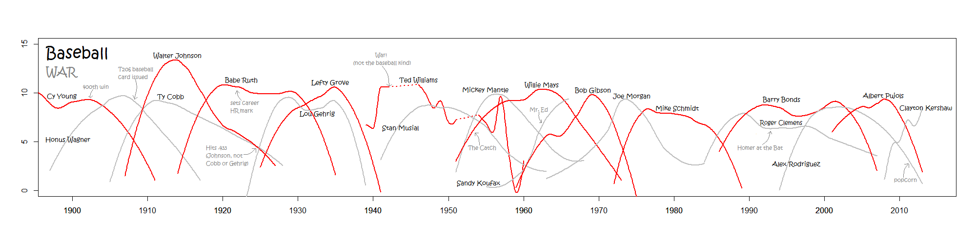
Why hierarchical clustering? Well, for one thing, it just looks really cool:

That right there is a dendrogram showing a clustering of all player-seasons since the year 2000. “Leaf” nodes on the left side of the diagram represent the seasons, and the closer together, the more similar they are. To create such a thing you first need to define “features” — essentially the points of comparison we use when comparing players. For this, I’ve just used basic statistics any casual baseball fan knows: AVG, HR, K, BB, and SB. We could use something more advanced, but I don’t see the point — at least this way the results will be somewhat interpretable to anyone. Plus, these stats — while imperfect — give us the gist of a player’s game: how well they get on base, how well they hit for power, how well they control the strike zone, etc.

Now hierarchical clustering sounds complicated — and it is — but once we’ve made a custom leaderboard here at FanGraphs, we can cluster the data and display it in about 10 lines of Python code.

import pandas as pd
from scipy.cluster.hierarchy import linkage, dendrogram
# Read csv
df = pd.read_csv(r'leaders.csv')
# Keep only relevant columns
data_numeric = df[['AVG','HR','SO','BB','SB']]
# Create the linkage array and dendrogram
w2 = linkage(data_numeric,method='ward')
labels = tuple(df.apply(lambda x: '{0} {1}'.format(x[0], x[1]),axis=1))
d = dendrogram(w2,orientation='right',color_threshold = 300)


Let’s use this to create some player comps, shall we? First let’s dive in and see which player-seasons are most similar to Mike Trout’s 2016:

Remember Bobby Abreu? He’s on the Hall of Fame ballot next year, and I’m not even sure he’ll get 5% of the vote. But man, take defense out of the equation, and he was Mike Trout before Mike Trout. The numbers are stunningly similar and a sharp reminder of just how unappreciated a career he had. Also Shin-Soo Choo is here.

So Abreu is on the short list of most underrated players this century, but for my money there is someone even more underrated, and it certainly pops out from this clustering. Take a look at the dendrogram above — do you see that thin gold-colored cluster? In there are some of the greatest offensive performances of the past 20 years. Barry Bonds’s peak is in there, along with Albert Pujols’s best seasons, and some Todd Helton seasons. But let’s see if any of these names jump out at you:

First of all, holy hell, Barry Bonds. Look at how far separated his 2001, 2002 and 2004 seasons are from anyone else’s, including these other great performances. But I digress — if you’re like me, this is the name that caught your eye:

Brian Giles had seven seasons that, according to this method at least, are among the very best this century. He had an elite combination of power, batting eye, and a little bit of speed that is very rarely seen. Yet he didn’t receive a single Hall of Fame vote, for various reasons (short career, small markets, crowded ballot, PED whispers, etc.) He’s my vote for most underrated player of the 2000s.

This is just one application of hierarchical clustering. I’m sure you can think of many more, and you can easily do it with the code above. Give it a shot if you’re bored one offseason day and looking for something to write about.

A little while back, I took a look at what might be considered the least likely home run of the 2016 season. I ended up creating a simple model which told us that a Darwin Barney pop-up which somehow squeaked over the wall was the least likely to end up being a homer. But what about the converse? What if we looked at the ball that was most likely to be a homer, but didn’t end up being one? That sounds like fun, let’s do it. (Warning: GIF-heavy content follows.)

The easy, obvious thing to do is just take our model from last time and use it to get a probability that each non-homer “should” be a home run. So let’s be easy and obvious! But first — what do you think this will look like? Maybe it was robbed of being a home run by a spectacular play from the center fielder? Or maybe this fly ball turned into a triple in the deepest part of Minute Maid Park? Perhaps it was scalded high off the Green Monster? Uh, well, it actually looks like this.

That’s Byung-ho Park, making the first out of the second inning against Yordano Ventura on April 8. Just based off exit velocity and launch angle, it seems like a worthy candidate for the title, clocking in at an essentially ideal 110 MPH with a launch angle of 28 degrees. For reference, here’s a scatter plot of similarly-struck balls and their result (click through for an interactive version):

(That triple was, of course, a triple on Tal’s hill)

But, if you’re anything like me, you’re just a tad underwhelmed at this result. Yes, it was a very well-struck ball, but it went to the deepest part of the park. What’s more, Kauffman Stadium is a notoriously hard place to hit a home run. It really feels like our model should take into consideration both the ballpark in which the fly ball was hit, and the horizontal angle of the batted ball, no? Let’s do that and re-run the model.

One tiny problem with this plan is that Statcast doesn’t actually provide us with the horizontal angle we’re after. Thankfully Bill Petti has a workaround based on where the fielder ended up fielding the ball, which should work well enough for our purposes. Putting it all together, our code now looks like this:

# Read the data
my_csv <- 'data.csv'
data_raw <- read.csv(my_csv)
# Convert some to numeric
data_raw$hit_speed <- as.numeric(as.character(data_raw$hit_speed))
data_raw$hit_angle <- as.numeric(as.character(data_raw$hit_angle))
# Add in horizontal angle (thanks to Bill Petti)
horiz_angle <- function(df) {
angle <- with(df, round(tan((hc_x-128)/(208-hc_y))*180/pi*.75,1))
angle
}
data_raw$hor_angle <- horiz_angle(data_raw)
# Remove NULLs
data_raw <- na.omit(data_raw)
# Re-index
rownames(data_raw) <- NULL

# Make training and test sets
cols <- c(‘HR’,’hit_speed’,’hit_angle’,’hor_angle’,’home_team’)
library(caret)
inTrain <- createDataPartition(data_raw$HR,p=0.7,list=FALSE)
training <- data_raw[inTrain,cols]
testing <- data_raw[-inTrain,cols]
# gbm == boosting
method <- ‘gbm’
# train the model
ctrl <- trainControl(method = “repeatedcv”,number = 5, repeats = 5)
modelFit <- train(HR ~ ., method=method, data=training, trControl=ctrl)
# How did this work on the test set?
predicted <- predict(modelFit,newdata=testing)
# Accuracy, precision, recall, F1 score
accuracy <- sum(predicted == testing$HR)/length(predicted)
precision <- posPredValue(predicted,testing$HR)
recall <- sensitivity(predicted,testing$HR)
F1 <- (2 * precision * recall)/(precision + recall)

print(accuracy) # 0.973
print(precision) # 0.811
print(recall) # 0.726
print(F1) # 0.766

Great! Our performance on the test set is better than it was last time. With this new model, the Park fly ball “only” clocks in at a 90% chance of becoming a home run. The new leader, with a greater than 99% chance of leaving the yard with this model is ARE YOU FREAKING KIDDING ME

I bet you recognize the venue. And the away team. And the pitcher. This is, in fact, the third out of the very same inning in which Byung-ho Park made his 400-foot out. Byron Buxton put all he had into this pitch, which also had a 28-degree launch angle, and a still-impressive 105 MPH exit velocity. Despite the lower exit velocity, you can see why the model thought this might be a more likely home run than the Park fly ball — it’s only 330 feet down the left-field line, so it takes a little less for the ball to get out that way.

Finally, because I know you’re wondering, here was the second out of that inning.

This ball was also hit at a 28-degree launch angle, but at a measly 102.3 MPH, so our model gives it a pitiful 81% chance of becoming a home run. Come on, Kurt Suzuki, step up your game.

Bryce Harper just had a down season. That seems like a weird thing to write about someone who played to a 112 wRC+, but when you’re coming off a Bondsian .330/.460/.649 season, a line of .243/.373/.441 seems pedestrian. Would most major-league baseball players like to put up a batting line that’s 12% better than average? Yes (by definition). But based on his 2015 season, we didn’t expect “slightly above average” from Bryce Harper. We expected “world-beating.” We didn’t quite get it, but there’s one thing he is still amazing at — no one in the National League can work the count quite like him.
Read the rest of this entry »

Canadians! They walk among us, only revealing themselves when they say something like “out” or “sorry” or “I killed and field-dressed my first moose when I was six.” But we don’t get to hear baseball players talk that often, so how can we tell if a baseball player is Canadian? Generally there are three warning signs:

1. They have a vaguely French-sounding last name
2. They have been pursued by the Toronto Blue Jays¹
3. They bat left-handed and throw right-handed

¹ I honestly thought Travis d’Arnaud was Canadian until just now

Wait, hold on. What’s up with that third one? This merits a bit of investigation.
Read the rest of this entry »

Have you heard of Michael Lorenzen?  You might have heard of Michael Lorenzen.  You’re a baseball fan, and he plays baseball.  But chances are, you haven’t heard of him.  He’s a mostly unremarkable relief pitcher for a very unremarkable Cincinnati team.  He put up a 2.88 ERA with a 3.67 FIP for the Reds in 2016, hurt by a 22.7% HR/FB rate.  But he did do something special last year, and that something special is worth noting.  Before getting into that, though, let’s take a trip to the distant past of 2009.
Read the rest of this entry »

Jeff recently ran two articles about the season’s worst and best home runs, as measured by exit velocity.  As a small addendum to that, I’d like to include both exit velocity and launch angle to try to determine the season’s least likely home run.  So how do we do such a thing?  Warning!  I’m going to spend a bunch of time talking about R code and machine learning.  If you want to skip all that, feel free to scroll down a bit.  If, on the other hand, you’d like a more in-depth look at running machine learning on Statcast data, hit me up in the comments and I’ll write some more fleshed-out pieces.

As usual, we’re going to rely heavily on Baseball Savant.  Thanks to their Statcast tool, we can download enough information to blindly feed into a machine-learning model to see how exit velocity and launch angle affect the probability of getting a home run.  For instance, if we wanted to make a simple decision tree, we could do something like this.

# Read the data
my_csv <- 'hr_data.csv'
data_raw <- read.csv(my_csv)
# Make training and test sets
library(caret)
inTrain <- createDataPartition(data_raw$HR,p=0.7,list=FALSE)
training <- data_raw[inTrain,]
testing <- data_raw[-inTrain,]
# rpart == decision tree
method <- 'rpart'
# train the model
modelFit <- train(HR ~ ., method=method, data=training)
# Show the decision tree
library(rattle)
fancyRpartPlot(modelFit$finalModel)

That looks like what we would expect.  To hit a home run, you want to hit the ball really hard (over 100 MPH) and at the right angle (between 20 and 40 degrees).  So far so good.

Now, decision trees are pretty and easy to interpret but they’re no good for what we want to do because (a) they’re not as accurate as other, more sophisticated methods and (b) they don’t give meaningful probability values.  Let’s instead use boosting and see how well we did on our test set.

method <- 'gbm' # boosting
modelFit <- train(HR ~ ., method=method, data=training)
# How did this work on the test set?
predicted <- predict(modelFit,newdata=testing)
# Accuracy, precision, recall, F1 score
accuracy <- sum(predicted == testing$HR)/length(predicted)
precision <- posPredValue(predicted,testing$HR)
recall <- sensitivity(predicted,testing$HR)
F1 <- (2 * precision * recall)/(precision + recall)

print(accuracy) # 0.973
print(precision) # 0.792
print(recall) # 0.657
print(F1) # 0.718

The accuracy number looks nice, but the precison and recall show that this is far from an amazingly predictive algorithm.  Still, it’s decent, and all we really want is a starting point for the conversation I started in the title, so let’s apply this prediction to all home runs hit in 2016.

Once you throw out some fairly clear blips in the Statcast data, the “winner”, with a 0.3% chance of turning into a home run, is this beauty from Darwin Barney.*  This baby had an exit velocity of 91 MPH and launch angle of 40.7 degrees.  For fun, let’s look at where similarly-struck balls in the Rogers Centre ended up this year.

* I’m no bat-flip expert, but I believe you can see more of a flip of “I’m disgusted” than “yay” in that clip.

Congrats Darwin Barney!  There are no-doubters, then there are maybes, and then there are wall-scrapers.  They all look the same in the box score, but you can’t fool Statcast.

With apologies to Randall Munroe:

Click to embiggen

If you’d like to make your own graph like this one, I’ve pasted the R code I used here.

I found Jeff’s recent post on Jake Arrieta fascinating, because he goes into a game and pulls out Arrieta’s eight worst pitches from that game. This is something I’d never really thought deeply about before. We all know what bad pitches look like, right? An 0-2 fastball down the heart of the plate, a hanging slider, a pitch in the dirt on a full count, sure. But can we quantify this? Is there a way to say mathematically (in a way that makes some sort of sense) whether one pitch was better than another? Follow me beyond the jump and I’ll share some thoughts about how we might do this.
Read the rest of this entry »

You, being an internet-reading baseball fan who even occasionally ventures into FanGraphs’s Community Research articles, have almost certainly heard of Enos Slaughter, and not just because of his multiple appearances in crosswords. You also may know that he is probably best-known for his Mad Dash, in which he raced home from first base in a World Series game on what was charitably ruled a double, but what many observers believe should have been ruled a single^{[citation needed]}. Scoring from first on a single — I bet that’s pretty rare, right? After all, one such case of it got its own Wikipedia page!

Well, according to Retrosheet, a runner scored from first on a single 16 times last year (not counting plays on which an error was charged). It’s already happened at least once this year. So if we’re talking about unlikely ways to score from first base, this doesn’t really qualify as “rare.”

You know what is rare? This is rare.

Read the rest of this entry »

This is part three of a three-part series detailing a method of judging pitch framing based on the prior probability of the pitch being called a strike.  In part 1, we motivated the method.  In part 2, we formalized it. Here in part 3, we look at the hitter’s effect on ball and strike calls.

The formula we’ve been using for judging catcher framing is the very simple

IsCalledStrike - prob(CalledStrike)

where IsCalledStrike is simply 1 if the pitch is called a strike, and 0 otherwise.  The second term is the probability that the pitch would have been called a strike, absent any information about any given party’s involvement. We add up these values for every called ball or strike that a catcher receives, and report the resulting number.  In this article we could go ahead and do this for all catchers over the past two years, except (a) Matthew Carruth is already doing this exact thing and (b) I can’t figure out how to match Retrosheet data to my Pitch F/X data to get catcher information anyway.  So instead we’ll look at hitter involvement.  How much can a hitter influence whether a pitch is called a ball or strike?

Read the rest of this entry »