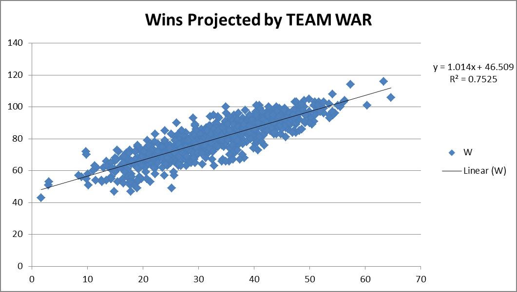
When I think of WAR, I tend to think of it truly in terms of wins. So when I see that a player is rated an 8 WAR player, to me I’m literally thinking this guy will get my team approximately eight additional wins. Otherwise we should really just rename this “best player metric.” Not that anything is wrong with a best player metric, but let’s not try to “connect” it to wins, if it’s not really connecting to wins, right? So I wanted to see how accurate this really is. So I downloaded the team WAR data from FanGraphs from 1985 – 2013, both hitting and pitching. I summed up the hitting & pitching WAR and plotted them versus the teams’ wins that year, hoping for a strong correlation.
You can see from the chart above, a correlation of 0.7525 was recorded. Great! This also shows a replacement-level team is about a 46.5-win team. Not unreasonable. Things make sense.
So then I figured, maybe we could try to do this same drill, but instead of using complete team calculations, what if we used individual position components? Would that result in a more accurate result? It’s possible, since the sum of a team’s individual player WAR values is not necessarily representative of the team WAR calculation alone. So what would this look like? So I went to FanGraphs again and downloaded the same dataset, except by position this time, instead of by team. For example, I’ve linked the catcher data below.
I went through and built a comprehensive list, tagging each player’s position. For pitchers the FanGraphs link was comprehensive, so I determined the RP and SP tag by assigning anybody who had >75% of their games also be games-started, as a SP, and all others as RPs. In some cases players showed up in multiple categories (i.e. Mike Napoli was listed as a C and 1b in 2011). In those events, I simply equally split their total seasonal WAR evenly across however many positions. So if a 6 WAR player showed up as a C & 1b & DH in a single season, each position was credited with 2 WAR. This prevented double or triple-counting of players. So how did this work out?
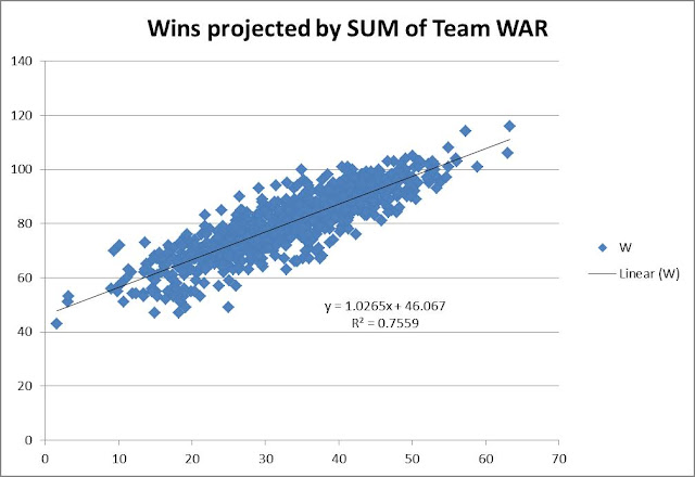
This actually projected slightly better. I do mean slightly — 0.7559 R2 versus the 0.7525 R2 when viewed as just team hitting and pitching. It also predicted basically the same replacement-level team, a 46-win one. So you could probably make the argument that it’s slightly more accurate to try to actually use the sum of the individual player WARs on the team instead of just a team calculation. But it is so close it’s probably not worth the extra effort for most exercises.
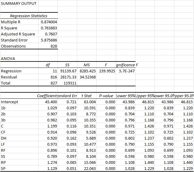
This then led me to think, why not try to tie wins in as a multi-variable regression using all the positions individually instead of just a linear one where we connect wins to some singular WAR total?
Since I already had the data i gave it a shot.
You can see here that we actually arrive at an R2 of a bit above 76%. So this is ever so slightly more predictive again. Again you also see that the intercept ends up very close to other methods, at 45.4 Wins for a replacement-level team. But bottom line, it’s basically as accurate as the other approaches. However, what I do find interesting in this approach is that it actually appears to value RP highest and the SS position the lowest. And those values are substantial. Very substantial.
You could probably make the argument then that shortstops are being overvalued by the present system. This could possibly mean the defensive position adjustment value for SS defense is too high. Reasons aside, this seems like a very legit finding, as the “WAR” metric appears to overstate SS value by 26.7% (1/0.789). So for example, a typical FanGraphs contract analysis approach can use a standard $/WAR value for projections into the future. Yet from this perspective, spending that $/WAR on a SS will have you significantly overweighting the benefit you’ll get from that SS. To a lesser extent that would also apply to 2b, CF and RFs.
Conversely, RP, SP and catcher figures are actually quite undervalued. This would certainly lend some credence to the approaches of “smaller” and “rebuilding” teams to date (think Royals and Astros, even last year’s Yankees) who have focused, among other things, on RP groups.
Based on this data, it would seem that focusing on pitching, specifically RP, and getting an excellent catcher, would be the best ways to focus on turning around a team. At least in the context of a singular $/WAR metric.
While this wasn’t what I went into this analysis looking for, it was a fairly surprising result. Yet one that seems to be in line with the approach many teams are currently taking.
NOTE: I do understand this could be refined even further to re-weight the players WAR values exactly correctly based upon their actual number of games at each position instead of the approach I took which was just to equally distribute those values. Given the size of that specific sample and what type of change we’d be talking about, I would find it unlikely that would move the needle substantially here though. But I think it’s an interesting finding.

Interesting. It is not surprising that RPs are underweighted by WAR when trying to find a linear relationship to Wins, because the higher leverage innings they pitch in are discounted in WAR (as opposed to WPA). Catcher WAR does not include framing (in Fangraphs) and other hard to measure attributes like game calling etc. Shortstop is more difficult to determine, but I suppose could be an overly aggressive position adjustment.
It’s possible, since the sum of a team’s individual player WAR values is not necessarily representative of the team WAR calculation alone.
Why not? Rounding errors might throw the totals off a little, but unless you’re including WAR that the players accrued while with other teams the team WAR should be sum of the players’ WAR.
So if a 6 WAR player showed up as a C & 1b & DH in a single season, each position was credited with 2 WAR.
That seems like it’s going to introduce some biases, though I’m not sure what the effects would be. E.g. if there are more catchers who occasionally play 1B than first basemen who occasionally play catcher then you’ll overestimate the amount of 1B WAR compared to catcher WAR. That would make each catcher win look more valuable than each 1B win, i.e. the coefficient for catchers would be higher than 1B. I’d be a bit reluctant to draw any conclusions about the value of individual positions without fixing this.
This could possibly mean the defensive position adjustment value for SS defense is too high.
I don’t think that works. All teams play one shortstop per game, so they all have the same positional adjustment over the season (or near enough – extra innings will change things slightly). Reducing the SS positional adjustment would just move all points on a wins versus SS WAR graph to the left, and so won’t change the slope.
Paul,
I actually went back and tried to address the positional WAR allocation issue that you noted above in your 2nd point, and i noted in my original post in my closing “NOTE”. I used fangraph’s defensive tables of statistics to identify the innings played by guys at various positions. The data only went back through 2002 though, so i had to shrink my analysis down from 85-2013 to 02-13.
The results were actually a bit different, SS is still overvalued significantly but 2b becomes the biggest loser now. However, this appears to really be driven by the time period change, not the positional precision. I also went back and ran the same regression on my “quick and dirty” positional data set and changed the time frame from ’85 to ’02, and i actually ended up with an almost identical output as the more accurate innings based approach.
So the real question from that is what’s more relevant to today’s game? Data from ’85 on or data from ’02 on. Probably ’02.. I’ve pasted in the regression output from the more accurate approach below, so you can see the different coefficients that resulted.
Regression Statistics
Multiple R 0.90680
R Square 0.82229
Adjusted R Square 0.81668
Standard Error 4.99226
Observations 360
ANOVA
df SS MS F Significance F
Regression 11 40132.65081 3648.422801 146.3900242 2.9002E-123
Residual 348 8673.071415 24.92261901
Total 359 48805.72222
Coefficients Standard Error t Stat P-value Lower 95% Upper 95% Lower 95.0% Upper 95.0%
Intercept 46.43984 0.94401 49.19428 0.00000 44.58316 48.29652 44.58316 48.29652
C 1.20847 0.15505 7.79415 0.00000 0.90352 1.51342 0.90352 1.51342
1b 1.17825 0.12268 9.60423 0.00000 0.93697 1.41954 0.93697 1.41954
2b 0.64468 0.14053 4.58753 0.00001 0.36829 0.92107 0.36829 0.92107
SS 0.86278 0.13755 6.27252 0.00000 0.59225 1.13331 0.59225 1.13331
3b 0.84767 0.12303 6.89010 0.00000 0.60570 1.08964 0.60570 1.08964
RF 0.78101 0.14425 5.41413 0.00000 0.49729 1.06473 0.49729 1.06473
CF 0.97481 0.12792 7.62067 0.00000 0.72322 1.22640 0.72322 1.22640
LF 0.78623 0.12876 6.10640 0.00000 0.53299 1.03947 0.53299 1.03947
DH 1.12481 0.25521 4.40745 0.00001 0.62287 1.62675 0.62287 1.62675
RP 1.43323 0.11228 12.7619 0.00000 1.21241 1.65406 1.21241 1.65406
SP 1.12974 0.06683 16.9052 0.00000 0.99829 1.26119 0.99829 1.26119
If you’re interested in what i did there, and fangraphs allows me to link to it, i have a more detailed post on my blog about that specific topic.
http://saber-fighters.blogspot.com/2016/03/war-by-position-update.html
Paul,
You are correct in your first point. It’s basically just a rounding issue. In the end this isn’t really relevant to the point of the article though. As my first two analysis were basically the exact same, which is I believe what you are alluding to.
With regards to your second comment, you may have noticed that you just restated my Note at the end of the post. That data all broken out by innings or outs isn’t as easy to come by with a lot of copy pasting, at least for an ameuter like myself, so doing said analysis is a bit tougher for the armchair analyst. Though I don’t think the impact would be too significant. You seem to disagree, but in particular with SS I would expect that’s the position where guys just moving around playing a few innings here and there would be the most unlikely. I.e. The position with the biggest impact here is probably the most unlikely to be impacted by a defensive committee approach. I’m only anecdotally assuming that as I don’t have the data though.
Your last point I about SS positional adjustments is not correct, at least as far as I understand the way they apply the adjustment. It’s not comparative between just shortstops but it’s a value reflective of the SS position vs other positions. Reducing the position adjustment would lower the SS runs saved which would then translate to lower SS war value while keeping other positions WAR the same.
What worried me about the even split of WAR for multi-position players was that I’d expect there to be persistent patterns of how players move between positions, which would prevent sample size from fixing the issue. To put it another way: sample size helps with noise, but the potential issue here was bias.
On the position adjustment: if I understand correctly your results suggest that if a team replaces a 2 WAR shortstop with a 3 WAR shortstop it would expect to gain 0.789 wins. If you reduce the SS position adjustment from +7.5 to, say, +2.5 runs, then the team is replacing a 1.5 WAR shortstop with a 2.5 WAR shortstop. That’s still a 1 WAR change and still a 0.789 extra expected wins, so the slope doesn’t change (though the intercept does). The slope being less than 1 implies that we’re somehow over-estimating the differences between shortstops.
Your 2nd point is easier to address. You’re just skipping the step where you have to re-calculate the new regression equation. the current regression equation would no longer apply to the adjusted SS war calculation. to break it down:
“if a team replaces a 2 WAR shortstop with a 3 WAR shortstop it would expect to gain 0.789 wins. ” – yes (though this is the 85-13 data. 02-13 says 0.862)
“If you reduce the SS position adjustment from +7.5 to, say, +2.5 runs, then the team is replacing a 1.5 WAR shortstop with a 2.5 WAR shortstop.” — yes, using the 10R per win thumb rule.
“That’s still a 1 WAR change and still a 0.789 extra expected wins, so the slope doesn’t change (though the intercept does).” — No. This is where you’re missing a key step. The regression equation that resulted in the 0.789 coefficient for that variable is based on the original SS WAR values. These being the WAR values calculated using the +7.5 adjustment. If a reduced position adjustment was applied then new WAR values for the SS position would be calculated for all SSs within the dataset. This new SS WAR value would be used to develop a new regression equation. Since we’d be lowering the overall WAR value for all SS, this should bring the regression coefficient up, closer to 1, for SS’s while leaving other positions unchanged.
“The slope being less than 1 implies that we’re somehow over-estimating the differences between shortstops.” – this is not true. the slope being less than 1 implies that we’re over-estimating the value of SS WAR with regards to it’s relationship with real wins as compared to other positions.
And that’s the whole point of this, to say that the current WAR equation when used by position to forecast actuals wins, only values SS WAR at 0.789 (0.86 in the 02-13 dataset). WAR is a stat that’s supposed to be equally applicable to all positions. This regression would show that’s in fact not true; ergo, as an equalizer across positions SS WAR is overestimated. Since much of WAR is entirely universal across positions (think standard offensive stats), really the only way it could be undervalued is things which are not applied in the same way (think fielding stats, think positional adjustment in particular as something that jumps out as a position unique WAR adjustment).
I guess i’m still a bit confused about your bias concern. I did recognize the possibility that results could get skewed by not having an exact breakdown of the percentage of time played at each position by players in my initial analysis. However, my feeling was that the sample size of players where this is a significant case would be largely insignificant to the regression. It turns out, at least using the data from 2002-now, i believe i was correct in my assumption that it wouldn’t be a big deal. An equal distribution by player alone, vs my redone approach using a weighted % by innings for each position yielded virtually the same regression. So if that was your point, and i agree that was a valid possible concern, the data appeared to put that issue to rest. THe approaches were very similar in the output, but sure if you can, use the more exact data. There still exists the possibility that a player may generate better offensive WAR when he’s a DH then when he’s a 3b or something, that’d be another possible issue since even though now that i’ve distributed the WAR by close to exactly the correct %% by position, that still assumes the WAR is generated equally by the player whenever any position is played. But i would expect that effect to be even smaller than the exact position inning impact, and the position inning impact was negligible, so this would probably be negligible as well.
I appreciate the comments!
Re-running the regression after reducing the SS position adjustment shouldn’t, as far as I can see, change the SS WAR co-efficient. Every team gets the same contribution to its WAR from the SS position adjustment (*), so you can think of team SS WAR (or any other position’s WAR) as a variable part (batting, running, fielding) plus a constant (position adjustment). If you reduce the constant by 0.5 WAR that shouldn’t affect the slope because that only depends on the variable part – instead, it should just increase the intercept from 45.4 to about 45.8 (0.5 X 0.789 ~= 0.4). That give a regression equation that makes exactly the same predictions as the original and hence has the same RMSE. If there’s a better set of co-efficients then they’d also be better with the original SS WAR simply by reducing the intercept, so the original regression should have found them.
Thanks for re-running with a more precise positional split; it’s somewhat comforting to see that it doesn’t change the results much. I wonder if the differences between the smaller and larger samples is due to the defensive metric being different for earlier years – TZ before 2002 and UZR from 2002 onwards. If so it might be best to stick to 2002-present to keep the metrics consistent.
(*) Or very close. Last year it varied from 7.3 to 7.5 runs – http://www.fangraphs.com/leaders.aspx?pos=all&stats=bat&lg=all&qual=0&type=6&season=2015&month=38&season1=2015&ind=0&team=0,ts&rost=0&age=0&filter=&players=0
Paul I believe you are over thinking it and making it too difficult. Take a simple example. Two variables where y equals 1+ 0. 5x.
5 3.5
3 2.5
8 5
The linear regression equation will be
0.5x + 1
If you then modified your data set with that insight to apply a factor of 0.5 to each x variable your new x & y values would be
2.5 3.5
1.5 2.5
4 5
And your new regression equation would be
X + 1
The coefficient for X changes not the intercept.
This is in essence exactly what I’m doing here. I think you are thinking too much into it.
The intercept doesn’t change in the regression.
I have done the exercise in the analysis workbook I’ve used. If I apply the coefficient to each specific position for the whole dataset and rerun the regression all the coefficients for each position become 1 and the intercept stays the same. This then means that each WAR rating is then truly an additional Win for a team.
I’m not a stats teacher or anything, so hopefully this is clear. Thanks again for the dialog!
Yes, if you multiply all your x values by a constant that will change the slope. However, that isn’t what changing a position adjustment will do. You don’t calculate a position-neutral WAR and then multiply by a position adjustment; instead, you add the position adjustment to the WAR. For individual players the adjustment varies proportionally to time spent at the position, but here we’re interested in teams. All teams play the same number of games, and they play one shortstop per game, so the SS position adjustment for every team is the same give or take a couple of tenths of a run. If you reduce the SS position adjustment down by, say, 0.5 wins you’re not multiplying the SS WAR by 0.5, you’re simply reducing it by 0.5. To use your example you’re going from:
5 3.5
3 2.5
8 5
to
4.5 3.5
2.5 2.5
7.5 5
The new equation is 0.5x + 1.25. Adding a constant changes the intercept, not the slope. So to go back to my original point, this statement:
This could possibly mean the defensive position adjustment value for SS defense is too high.
cannot be the explanation for your results. That leaves the question: what is the explanation?
1) Multicollinearity. As I understand it (I’m not a statistician either) multiple regression can get confused if the independent variables are correlated with each other. So if there’s a tendency for good players to play with other good players, e.g. because high payroll teams can afford multiple good players, the regression will have difficulty assigning the results to individual positions. It would be worth checking for this if you haven’t already.
2) Defensive metrics. We know that UZR contains some measurement error that means we ought to regress the reported values to estimate what actually happened. If some positions need more regression than others then WAR would exaggerate the differences between players at those positions more than others. Would that be enough to account for 1B wins being 80% more valuable than 2B wins though? And why would corner outfield positions be so different from CF? This explanation makes some sense but feels unsatisfactory.
3) Something else. I think this is the most likely option, it’s just not very helpful. 🙂
I would agree that i think #3 “something else” is the most likely option and is the explanation. I think a part of that something is very likely defensive metrics. Maybe middle infielders and corner OFs are getting too much credit, whereas the hits to 1b and DHs are over-magnified.
I understand your point regarding the slope/intercept. We were not on the same page there because i by no means meant to imply the only thing that could be used to do the explanation is defensive metrics. Simply as a part of the explanation for why certain positions could be under/over valued. Thereby allowing for the use of the regression coefficient to either increase or decrease the value.
I’m unsure what the overall reason is, but i also think it’s an interesting topic. It would seem to me that when WAR is viewed as a value that can be tied to a $$$$$, like $7m/win or $8/win, to evaluate/estimate a contract this is something that’s important to understand. In order to do that you need to ensure WAR is really equal to a Win, and it would appear that at corner outfield and middle infield positions, the present formula for calculating WAR does not generate that. I’m not sure how the standard analysis went for corner outfielder analysis on contracts like Alex Gordon and Jason Heyward this year, but it’s interesting to note that this approach would say those guys are worth closer to 5.5-6m per Win if you apply the ~25% corner OF reduction.
i appreciate your feedback. it’s just a topic i found interesting.