Archive for wOBA

Examining the foundations of batting analysis began in Part 1 with an historical examination of the earliest statistics designed to examine the performance of batters. In Part 2, I presented a new method for calculating basic averages reflecting the “real and indisputable” rate at which batters reached base. In Part 3, I examined the development of run estimation techniques over the last century, culminating with the linear weights system. I will employ that system now as I reconstruct run estimation from the bottom up.

We use statistics in baseball to tell stories. Statistics describe the action of the game or the performance of players over a period of time. Statistics inform us of how much value a player provided or how much skill a player showed in comparison to other players. To tell such stories successfully, we must understand how the statistics we use are constructed and what they actually represent.

A single, for instance, seems simple enough at first glance. However, there are details in its definition that we sometimes gloss over. In general, a single is any event in which the batter puts the ball into play without causing an out, while showing an accepted form of batting effectiveness (reaching on a hit), and ultimately advancing to first base due to the primary action of the event (before any secondary fielding errors or advancement on throws to other bases). Though this is specific in many regards, it is still quite a broad definition for a batting event. The event could occur in any inning, following any number of outs, and with any number of runners on the bases. The ball could be hit in any direction, with any speed and trajectory, and result in any number of baserunners advancing any number of bases.

These kinds of details form the contextual backdrop that characterizes all batting events. When we construct a statistic to evaluate these events, we choose what level of contextual detail we want to consider. These choices define our analysis and are critical in developing the story we want to tell. For instance, most statistics built to measure batting effectiveness—from the simple counting statistics like hits and walks, to advanced run estimators like Batter Runs or weighted On Base Average (wOBA)—are constructed to be independent of the “situational context” in which the events occur. That is, it doesn’t matter when during the game a hit is made or if there are any outs or any runners on the bases at the time it happens. As George Lindsey noted in 1963, “the measure of the batting effectiveness of an individual should not depend on the situations that faced him when he came to the plate.”

Situational context is the most commonly cited form of contextual detail. When a statistic is described as “context neutral,” the context being removed is very often the one describing the out/base state before and after the event and the inning in which it occurred. However, there are other contextual details that characterize the circumstances and conditions in which batting events occur that also tend to be removed from consideration when analyzing their value. Historically, where the ball was hit, as well as the speed and trajectory which it took to reach that location, have also not been considered when judging the effectiveness of batters. This has partly been due to the complexity of tracking such things, especially in the century of baseball recordkeeping before the advent of computers. Also, most historical batting analyses focus exclusively on the outcome for the batter, independent of the effect on other baserunners. If the batter hits the ball four feet or 400 feet but still only reaches first base, there is no difference in the personal outcome that he achieved.

If the value of a hit was limited to only how far the batter advances, then there would be no need to consider the “batted-ball context,” but as F.C. Lane observed in 1916, part of the value of making a hit is in the effect on the “runner who may already be upon the bases.” By removing the batted-ball context when considering types of events in which the ball is put into play, we’re assuming that a four-foot single and 400-foot single have the same general effect on other baserunners. For some analyses, this level of contextual detail describing an event may be irrelevant or insignificant, but for others—particularly when estimating run production—such a level of detail is paramount.

Let’s employ the linear weights method for estimating run production, but allow the estimation to vary from one completely independent of any contextual detail to one as detailed as we can make it. In this way, we’ll be able to observe how various details impact our valuation of events. Also, in situations where we are only given a limited amount of information about batting events, it will allow us to make cursory estimations of how much they caused their team’s run expectancy to change.

To begin, let’s define the run-scoring environment for 2013.[i] While we have focused on context concerning how events transpired on the field, the run scoring environment is another kind of contextual detail that characterizes how we evaluate those events. The exact same event in 2013 may not have caused the same change in run expectancy as it would have in 2000 when runs were scored at a different rate. We will define the run scoring environment for 2013 as the average number of runs that scored in an inning following a plate appearance in each of the 24 out/base states – a 2013-specific form of George Lindsey’s run expectancy matrix:

While we will focus on examining various levels of contextual detail concerning the events themselves, the run-scoring environment can also be varied based on contextual details concerning the scoring of runs. The matrix we will employ, as defined by Lindsey, reflects the average number of runs scored across the entire league. If we wanted, we could differentiate environments by league or park, among other things, to try and reflect a more specific estimate of the number of runs produced. As the work I’m going to present is meant to provide a general framework for run estimation, and these adjustments are not trivial, I’m going to stick with the basic model provided by Lindsey.

With Lindsey’s tool, we can define a pair of statistics for general analysis of run production. Expected Runs (xR) reflect the estimated change in a team’s run expectancy caused by a batter’s plate appearances independent of the situational context in which they occur. A batter’s expected Run Average (xRA) is the rate per plate appearance at which he produces xR.

xRA = Expected Runs / Plate Appearances = xR / PA

xR and xRA create a framework for estimating situation-neutral run production. Based on the contextual specificity that is used to describe the action of a plate appearance, xR and xRA will yield various estimations. The base case for calculating expected runs, xR₀, is calculated independently of any contextual detail, considering only that a plate appearance occurred. By definition, an average plate appearance will cause no change in a team’s run expectancy. Consequently, no matter a player’s total number of plate appearances, his xR₀ and, by extension, his xRA₀, will be 0.0.

This is completely uninformative of course, as base cases often are. So let’s add our first layer of contextual specificity by noting whether an out occurred due to the action of the plate appearance. This is the most significant contextual detail that we consider when evaluating batting events – it is the only factor that determines whether a plate appearance increases or decreases a team’s run expectancy. In 2013, 67.5 percent of all plate appearances resulted in at least one out occurring. On average, those events caused a team’s run expectancy to decrease by .252 runs. The 32.5 percent of plate appearances in which an out did not occur caused a team’s run expectancy to increase by .524 runs on average. We’ll define xR₁ as the estimated change in run expectancy based exclusively on whether the batter reached base without causing an out; xRA₁ is the rate at which a batter produced xR₁ per plate appearance.

You’ll notice that the components that construct xRA₁ can only take on two values—.524 and -.252—in the same way that the components that construct effective On Base Average (eOBA) (as defined in Part 2) can only take on two values—1 and 0. These statistics—xRA₁ and eOBA—have a direct linear correlation:

In effect, xRA₁ is a weighted version of eOBA, incorporating the same contextual details but on a different scale. This estimation provides us with an association between reaching base safely and producing runs. However, the lack of detail would suggest that all players that reach base at the same rate produce the same value, which is over simplified. It’s why you wouldn’t just use eOBA, or eBA, or any other basic statistic that reflects the rate which a batter reaches base, when judging the performance of a batter. Let’s add another layer of contextual detail to account for the different kinds of value a batter provides when he reaches base.

xR₂ will represent the estimated change in run expectancy based on whether the batter safely reached base and the number of bases to which he advanced due to the action of the plate appearance; xRA₂ will be the rate at which a batter produces xR₂ per plate appearance. While xR₁ and xRA₁ were built with just two components to estimate run production, xR₂ and xRA₂ require five components: one to define the value of an out, and four to define the value of safely reaching each base.

In 2013, a batter safely reaching first base during a plate appearance caused an average increase of .389 runs to his team’s run expectancy. Reaching second base was worth .748 runs, third base was worth 1.026 runs, and reaching home was worth 1.377 runs on average. Where xRA₁ provided a run estimation analog to eOBA, xRA₂ is built with very similar components to effective Total Bases Average (eTBA), though it’s not quite a direct linear correlation:

The reason xRA₂ and eTBA do not correlate with each other perfectly, like xRA₁ and eOBA, is because the way in which a batter advances bases is significant in determining how valuable his plate appearances were. Consider two players that each had two plate appearances: Player A hit a home run and made an out, Player B reached second base twice. Their eTBA would be identical—2.000—as they each reached four bases in two plate appearances. However, from the run values associated with reaching those bases, Player A would record 1.125 xR₂ from his home run and out, while Player B would record 1.496 xR₂ from the two plate appearances leaving him on second base. Consequently, Player A would have produced a lower xRA₂ (.5625) than Player B (.7480), despite their having the same eTBA. These effects tend to average out over a large enough sample of plate appearances, but they will still cause variations in xRA₂ among players with the same eTBA.

As stated in Part 2, the two main objectives of batters are to not cause an out and to advance as many bases as possible. If the only value that batters produced came from accomplishing these objectives, then we would be done – xR₂ and xRA₂ would reflect the perfect estimations of situation-neutral run production. As I hope is clear, though, the value of a batting event is dependent not only on the outcome for the batter but on the impact the event had on all other runners on base at the time it occurred. Different types of events that result in the batter reaching the same base can have different average effects on other baserunners. For instance, a single and a walk both leave the batter on first base, but the former creates the opportunity for baserunners to advance further on average than the latter. To address this, the next layer of contextual detail will bring the official scorer into the fray. xR₃ will represent the estimated change in run expectancy produced during a batter’s plate appearance based on:

(1)    whether the batter safely reached base,

(2)    the number of bases, if any, to which the batter advanced due to the action of the plate appearance, and

(3)    the type of event, as defined by the official scorer, that caused him to reach base or cause an out.

xRA₃ will, as always, be the rate at which a batter produces xR₃ per plate appearance.

Each of the run estimators that were examined in Part 3, from F.C. Lane’s methods through wOBA, are subsets of this level of xR. Expected runs incorporate estimations of the value produced during every event in which the batter was involved, including those which may be considered “unskilled.” The run estimators examined in Part 3 consider only those events that reflected a batter’s “effectiveness,” and either disregard the “ineffective” events or treat them as failures. xR₃ provides the total value produced by a batter, independent of the effectiveness he showed while producing it, based solely on how the official scorer defines the events. Consequently, some events, like strikeouts, sacrifice bunts, reaches on catcher’s interference, and failed fielder’s choices, among other more obscure occurrences, are examined independently in xR₃. From the two components of xR₂ and the five of xR₃, we build xR₄ with 18 components: five types of outs and 13 types of reaches.

To help illustrate how xR has progressed from level to level, here is a chart reflecting the run values for 2013 as estimated by xR based on the contextual detail provided thus far.

xR Progression

Beyond any consideration of skilled or unskilled production, xR₃ is the level at which most run estimators are constructed. It incorporates events that are well defined in the Official Rules of the game, and have been for at least the last few decades, and in some cases for over a century. While we still define most of a batter’s production by his accomplishing these events, we live in an era where we can differentiate between events on the field in more specific ways. Not all singles are identical events. We weaken our estimation of run production if we don’t account for the different kinds of singles, among other events, that can occur. xR₃ brought the official scorer into action; xR₄ will do the same with the stat stringer.

While the scorer is concerned with the result of an event, a stringer pays attention to the action in between the results. They chart the type, speed, and location of every pitch, and note the batted ball type (bunt, groundball, line drive, flyball, pop up) [ii] and the location to which the ball travels when put into play.While we don’t have this data as far back in time as we have result data, we do have decades worth of information concerning these details. By differentiating events based on these details, we will begin to unravel the “batted-ball context.” Ideally, we would know every detail of the flight of the ball, and use this to group together the most similar possible type of events for comparison.[iii] At present, we’re limited to what the scorers and stringers provide, but that’s still quite a lot of information.

xR₄ will represent the estimated change in run expectancy produced during a batter’s plate appearance based on:

(1)    whether the batter safely reached base,

(2)    the number of bases, if any, to which the batter advanced due to the action of the plate appearance,

(3)    the type of event, as defined by the official scorer, that caused him to reach base or make an out,

(4)    the type of batted ball, if there was one, as defined by the stat stringer, that resulted from the plate appearance,

(5)    the direction in which the ball travelled, and

(6)    whether the ball was fielded in the infield or outfield.

xRA₄ will be the rate at which a batter produces xR₄ per plate appearance.

There are 18 components in xR₃ which describe the assorted types of general events a batter can create.  When you add in these details concerning the batted-ball context, the number of components increases to 145 for xR₄. With such specific details being considered, we can no longer rely on a single season of data to accurately inform us on the average situation in which each type of event occurs; the sample sizes for some events are just too small. To address this, there are two steps required in evaluating events for xR₄. The first is to build a large sample of each event to build an accurate picture of their relative frequency in each out/base state. I’ve done this by using a sample covering the previous ten seasons to the one in which the estimations are being made. Once this step is completed, the run-scoring environment in the season being analyzed is applied to these frequencies, in the same way it is when looking at single season frequencies for basic events.

For instance, the single, which is traditionally treated as just one type of event, is broken into 24 parts based on the contextual details listed above. By observing the rate at which each of these 24 variations of singles occurred in each out/base state from 2004 through 2013, and applying the 2013 run-scoring environment, we get the following breakdown for the estimated value of singles in 2013:

This process is repeated for every type of batting event in which the ball is put into play. One of the ways we can use this information is to consider the run value based not on the result of the event, but on the batted-ball context that describes the event. Here are those values in the 2013 run-scoring environment:

Similarly, we can break down each player’s xR₄ by the value produced on each type of batted ball. Here are graphs for xR₄ produced on each of the four types of batted balls resulting from a swing, with respect to the number of batted balls of that type hit by the player. For simplicity, from this point on, when I drop the subscript when describing a batter’s expected run total, I’m referring to xR₄.

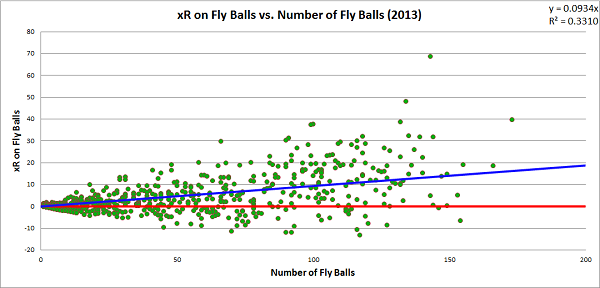
Line drives are the most optimal result for a batter. The first objective of batters is to reach base safely, and they did that on 67.0 percent of line drives last season. No batter who hit at least eight line drives in 2013 caused a net decrease in his team’s run expectancy during those events. For most batters, hitting the ball into the outfield in the air is the ideal way to produce value, as fly ball production tends to create a positive change in a team’s run expectancy. However, fly balls have the most variance of any of the batted ball types, and there are certainly batters who hurt their teams more when hitting the ball at a high launch angle than a low one. Here are the players to produce the lowest xRA on fly balls last season (minimum 50 fly balls):

For each of these batters, hitting the ball on the ground or on a line drive were far better results on average.

While groundballs may be a preferable result for some batters when compared to fly balls, they are still effectively batting failures for the team. There were 840 batters in 2013 to hit at least one groundball and only 44 produced a net positive change in their team’s run expectancy. Of those 44 players, only 11 hit more than 10 groundballs, and only two (Mike Trout and Juan Francisco) hit at least 100 groundballs. Here are the players with the highest xRA on groundballs in 2013 who hit at least 100 groundballs:

xR₄ allows us to tell the most detailed story concerning the type of value a batter produced, independent of the situational context at the time the plate appearance occurred. Because we gradually added layers of detail to our estimation, we can compare how each level of expected runs correlates to this most detailed level. In this way, we can judge how much information each level provides with respect to our most detailed estimation. Here is a graph that charts a batter’s xR₄ with respect to his xR₁, xR₂, and xR₃ estimations:

The line that cuts through the data reflects the xR₄ values charted against themselves. For each xR_n, we can calculate how well it correlates with xR₄ and, consequently, how much of xR₄ it can explain. Remember that we have already shown that xR₁ has a direct linear correlation with eOBA and xR₂ has a very high, though not quite direct, correlation with eTBA. For the xR₁ values, we observe a correlation, r, with xR₄ of .912, and an r² of .832, meaning that knowing the rate at which a batter reaches base explains over four-fifths of our estimation of xR₄. For the xR₂ values, r² increases to .986; for the xR₃ values, r² increases slightly higher to .990.[iv]

The takeaway from this is that when considering the whole population of players, there is little difference in a run estimator that considers the batted-ball context and one that does not; you can still explain 99 percent of the value estimated by xR₄ by stopping at xR₃. In fact, if all you know is the rate at which a batter accomplishes his two main objectives—reaching base and advancing as far as possible—you can explain well over 90 percent of the value estimated by xR₄. However, on an individual level, there is enough variation that observing the batted-ball context can be beneficial. Here are the five players with the largest positive and negative differences between their xR₃ and xR₄ estimations:

These changes are not massive, and these are the extreme cases for 2013, but they are certainly large enough that ignoring them will weaken specific analyses of batting production. Incorporating batted ball details into our analysis adds a significant layer of complexity to our calculation, but it must be considered if we want to tell the most accurate story of the value a batter produced.

If this work seems at all familiar, you may have read this article that I wrote last year on a statistic that I called Offensive Value Added (OVA). For all intents and purposes, OVA and xR are identical. I decided that the name change to xR would help me differentiate estimations more simply, as I could avoid naming four separate statistics for each level of contextual detail, but there was also a secondary reason for changing the presentation of the data. OVAr was the rate statistic associated with OVA, and it was scaled to look like a batting average, much in the same way that wOBA is scaled to look like an on base average. At the time, I choose to do this to make it easier to appreciate how a batter performed, since many baseball enthusiasts are comfortable interpreting the relative significant of a batting average.

After thinking on the subject, though, I came to decide that I prefer statistics that actually “mean” something to those that give a general, unit-less rating. For instance, try to explain what wOBA actually reflects. It starts as a run estimator, but then it’s transformed into a number that looks like a statistic with specific units (OBA), while not actually using those units. Once that transformation occurs, it no longer reflects anything specific and only serves as a way to rate batters. The same principle applies to other statistics as well, most notably OPS, which is arguably the most meaningless of all baseball statistics, perhaps all statistics ever (don’t get me started).

xR and xRA estimate the change in a team’s run expectancy caused by a batter’s plate appearances. They are measured in runs and runs per plate appearance, respectively. xRA may not look like a number you’ve seen before, and generally needs to be written out to four decimal places instead of three, unlike basic averages, but it’s linguistically very simple to use and understand. I’d rather sacrifice the comfort of having a statistic merely look familiar and instead have it actually reflect something tangible. This doesn’t take away from the value of a statistic like wOBA, which is a great run estimator no matter what scale it is on; a lack of meaning certainly does not imply a lack of value. Introducing an unscaled run average, xRA, will hopefully create a different perspective on how to talk about batting production.

There is one final expected run estimation that I want to consider that could easily cover an entire new part on its own, but I’ll limit myself to just a few paragraphs. The xR estimations we have built have been constructed independent of the situational context at the time of the batter’s plate appearance. Since we want to cover the entire spectrum of context-neutral run estimation to context-specific run estimation, we will conclude by considering xR_s, which is an estimate of the change in a team’s run expectancy based on the out/base state before and after the action of the plate appearance. This is very nearly the same thing as RE24 but it only considers runs produced due to the primary action of plate appearances and not baserunning events.

In many respects, xR_s is the simplest run estimator to construct of all that we have built thus far. There are only three pieces of information you need to know in a given plate appearance to construct xR_s: the run-scoring environment, the out/base state at the start of the action of the plate appearance, and the out/base state at the end of the action of the plate appearance. Next time you go to a baseball game, bring along a copy of a run expectancy matrix, like the one provided earlier. On a scorecard, at the start of every plate appearance, take note of the value assigned to the out/base state, making adjustments if any runners move while the batter is still in the batter’s box. Once the plate appearance is over, note the value of the new out/base state, separating out any advancement on secondary fielding errors or throws to other bases. Subtract the first value from the second value, and add in any RBIs on the play, and write the number in the box associated with the batter’s plate appearance; you just calculated xR_s. Do this for a whole game, and you will have a picture of the total value produced by every batter based on the out/base state context in which they performed.

The effective averages and expected run estimations provide a foundation on which batting analysis can be performed. They combine both “real and indisputable facts” with detailed estimations of the run produced in every event in which a batter participates. Any story that aims to describe the value that a batter provides to his team must consider these statistics, as they are the only ones which account for all value produced. 147 years ago, Henry Chadwick suggested that batters should be judged on whether they passed a “test of skill.” I think they should be judged on whether they passed a “test of value.”

Thanks to Benjamin H Byron for editorial assistance, as well as the staff at the Library of Congress for assistance in locating original copies of the 19^th century newspaper articles included in Part 1.

Here is data on eOBA, eTBA, and each level of xR and xRA estimation, for each batter in 2013.

Bibliography

[i] I’ll be focusing on 2013 because the full season is complete. All the work described here could easily be applied to 2014, or any other season, I just don’t want to use incomplete information.

[ii] While these terms are used a lot, there aren’t any specific definitions commonly accepted that differentiate each type of batted ball. For terms used so commonly, it doesn’t make much sense to me that they are not well defined. It won’t apply to the data used in this research, but here is my attempt at defining them.

A bunt is a batted ball not swung at but intentionally met with the bat. A groundball is a batted ball swung at that lands anywhere between home plate and the outer edge of the infield dirt and would be classified as a line drive if it made contact with a fielder in the air. A line drive is a batted ball swung at that leaves the bat at an angle of at most 20° above parallel to the ground (the launch angle), and either lands in the outfield or makes contact with any fielder before landing (generally through a catch, but sometimes a deflection). A fly ball is a batted ball swung at, with a launch angle between 20° and 60° above parallel (not inclusive), that either lands in the outfield or is caught in the air by a player in the outfield. A popup is a batted ball swung at that either (a) leaves the bat at an angle of 60° or greater above parallel and lands or is caught in the air in the outfield, or (b) leaves the bat at an angle greater than 30° and lands or is caught in the air in the  infield.

This would result in some balls being classified differently than they currently are, and not just because differentiating between a line drive and a fly ball is somewhat difficult with just a pair of eyes. If the defense were to play an infield shift, and the batter were to hit a line drive into the outfield grass into that shift, subsequently being thrown out at first base, it would likely be called a groundout by current standards. Batted balls should not be defined based on defensive success or failure, but by the general path which they take when leaving the bat. It may be unusual to credit a batter with making a line out despite the ball hitting the ground, but it more accurately reflects the type of ball put into play by the batter.

I don’t know that these are the “correct” ways to group together these events, but as we now are using technology that tracks the flight of the baseball from the moment it is released by the pitcher through the end of the play, we should probably have better definitions for types of batted balls than those currently provided by MLB. I don’t expect a human stringer to be able to differentiate between a ball hit with a 15° launch angle or a 25° launch angle, but that doesn’t mean we shouldn’t have some standard definition for which they should aim.

[iii] In theory, xR₅ would attempt to consider details that are even more specific, perhaps the initial velocity of the ball off the bat, the launch angle, and whatever other information can be gleaned from technology like HIT F/X. The xR framework leaves room to consider any further amount of detail that a researcher wants to consider.

[iv] Though not charted here, the r² value based on the correlation between wRAA, the “counting” version of wOBA, and xR₄ is .984. As wRAA is nearly identical to xR₃ but excludes a few of the more rare events from its calculation, it’s not surprising that the r² value between wRAA and xR₄ is just slightly smaller than the r² between xR₃ and xR₄.

In early May I introduced Ottoneu players to the Advanced Standings Dashboard, a tool that allows team owners to decipher the early season standings in an effort to better gauge where their team might be headed as the 2014 season comes together. You can download that tool here (http://goo.gl/pbXI5), but now that we’ve just entered July, the traditional halfway point of the baseball season, it’s time to take a deeper look at a few ways this tool can be used to effectively to manage your team into contention in the second half.

Since the tool can be updated easily with just a couple of copy/paste actions, I use this tool almost daily in my own FGPoints Ottoneu league.  But for fun, let’s walk through a few features as they apply to the FanGraphs Staff League, with a special focus on Eno Sarris’ team, “It’s A Perm“.

Eno enters July as a 3rd place team, nearly 400 points out of 1st place, and 150 out of 2nd.  In general, with at least seven teams over the 8,000 point mark, this league looks competitive at a glance.  But with the recent pickup of Ryan Braun, Eno clearly has his sights set on a title (https://twitter.com/enosarris/status/483016142831644672), so let’s break down the standings using the tool to see if Eno has the momentum to win it all in the 2nd half.

The first tab of the tool is simply the statistical breakdown of the Ottoneu standings into some common sabermetric calculations.  While we can easily see Eno leads the league offensively at 5.44 P/G, the underlying statistics also support it, showing he maintains an (slight) advantage in OPS, OPS+, wOBA, Runs Created, and Total Bases.  What may be more interesting is that Eno has more points scored from his offense than any other team in the league.  In fact, just over 58% of his points have come from his hitters (tab 3, ‘Projected Finish”). With roughly 55% of league scoring in Ottoneu coming from offense, Eno is clearly banking on this approach of shoring up the side of the ledger that carries the most weight.  The acquisition of Braun will only help.

So It’s A Perm is built on bats, but what about the pitching? Unfortunately, this is a weak spot, as Eno’s FIP, WHIP, and BB/9 are all higher than the two teams he’s chasing.  I’m sure he knows this instinctively as his 5.03 P/IP is below the league average of 5.13 P/IP (and further below the top 7 teams of 5.19 P/IP), but the dashboard makes it quicker and easier to point out these pitching deficiencies.  One possible area of improvement: the bullpen.  Without looking at his roster, I can tell you pretty quickly he’s probably pretty frustrated with his bullpen, which has been almost 42% less effective (“PEN” = Saves + Holds/IP) than the league leader, A Little Out of Context.  Shoring up a bullpen is often easier and cheaper than finding an ace SP mid season, so does Eno speculate on the eventual Sergio Romo replacement? Does he approach John Heyman’s Last Sirloin about shedding some of his bullpen pieces in a plea to “deal from strength”?

Once you’ve taken the time to digest some of the traditional sabermetric outputs in the Dashboard, your eyes will naturally gravitate toward the end of the first tab into the “League Projections” section, which is where the real power of the tool comes alive.  The key takeaways here are the “Otto” score and the “Pace” columns.  The Otto score can be better explained here by Chad Young (http://goo.gl/KK4Xy), while the “Pace” attempts to project the season-ending point totals for each team based up a range of factors, including current P/G and P/IP values, remaining IP and GP, and league averages in these areas.  In many leagues these are the columns that can better identify contenders from pretenders, but for the FanGraphs Staff league we see more evidence that the actual standings are, for the most part, very accurate, as Eno is also projected to end the season with the 3rd most points (18,042, or about 400 points out of 1st place).

There are a few interesting things to note here, however. First, John Heyman’s Last Sirloin actually has the third highest Otto score (13.66), but is still projected for 4th place, most likely due to his slower pace in IP (1,416 projected).  If this team can pick up the IP pace in the 2nd half with similar quality IP (5.54 P/IP), this team could make up ground quickly.  This team is clearly riding a league-best bullpen and trying to maximize its RP innings as much as possible.

Second, Ground Rule Double Helmet, despite sitting in 4th place with a strong 9,000 points, has had to overtax a very week pitching staff (4.74 P/IP) just to get there (1,577 IP projected).  The tool sees as much and projects this team to end the season in 5th place, but unless the pitching staff sees a significant improvement in the 2nd half, I’d expect this team to possibly fall even further as the season shakes out.

And that’s just the first tab…Once you get familiar with the tool, you’ll actually find the third tab, “Projected Finish” to be the most useful summary of some of these features described above, as it will give you a daily update of the projected champion for the league.  With Eno just 400 points out of both the actual and projected season-ending standings, this league is just too close to call on July 1st, but there are at least four clear contenders here, and It’s A Perm is one of them.  Will Ryan Braun help the cause? Just for fun, let’s say Braun increases Eno’s offense by just 2.00% (from 5.44 to 5.55).  Well, that could be all it takes, as that small increase moves the needle for It’s A Perm enough to overtake Johan Santa Claus by 100 points in the projected season-ending standings, and less than 200 points out from 1st place.  Of course, that’s if everything else stays the same, and, as in life, the only thing constant in baseball is change.  This will be a fun league to watch as the summer heats up, so enjoy the tool and use it where possible to get that 2% edge.

I’ve decided to break this final section in half and address the early development of run estimation statistics first, and then examine new ways to make these estimations next week. In Part 1, we examined the early development of batting statistics. In Part 2, we broke down the weaknesses of these statistics and introduced new averages based on “real and indisputable facts.” In Part 3, we will examine methods used to estimate the value of batting events in terms of their fundamental purpose: run creation.

The two main objectives of batters are to not cause an out and to advance as many bases as possible. These objectives exist as a way for batters to accomplish the most fundamental purpose of all players on offense: to create runs. The basic effective averages presented in Part 2 provide a simple way to observe the rate at which batters succeed at their main objectives, but they do not inform us on how those successes lead to the creation of runs. To gather this information, we’ll apply a method of estimating the run values of events that can trace its roots back nearly a century.

The earliest attempt to estimate the run value of batting events came in the March 1916 issue of Baseball Magazine. F.C. Lane, editor of the magazine, discussed the weakness of batting average as a measure of batting effectiveness in an article titled “Why the System of Batting Averages Should be Changed”:

“The system of keeping batting averages…gives the comparative number of times a player makes a hit without paying any attention to the importance of that hit. Home runs and scratch singles are all bulged together on the same footing, when everybody knows that one is vastly more important than the other.”

To address this issue, Lane considered the fundamental purpose of making hits.

“Hits are not made as mere spectacular displays of batting ability; they are made for a purpose, namely, to assist in the all-important labor of scoring runs. Their entire value lies in their value as run producers.”

In order to measure the “comparative ability” of batters, Lane suggests a general rule for evaluating hits:

“It would be grossly inaccurate to claim that a hit should be rated in value solely upon its direct and immediate effect in producing runs. The only rule to be applied is the average value of a hit in terms of runs produced under average conditions throughout a season.”

He then proposed a method to estimate the value of each type of hit based on the number of bases that the batter and all baserunners advanced on average during each type of hit. Lane’s premise was that each base was worth one-fourth of a run, as it takes the advancement through four bases for a player to secure a run. By accounting for all of the bases advanced by a batter and the baserunners due to a hit, he could determine the number of runs that the hit created. However, as the data necessary to actually implement this method did not exist in March 1916, the work done in this article was little more than a back-of-the-envelope calculation built on assumptions concerning how often baserunners were on base during hits and how far they tended to advance because of those hits.

As he wanted to conduct a rigorous analysis with this method, Lane spent the summer of 1916 compiling data on 1,000 hits from “a little over sixty-two games”[i] to aid him in this work. During these games, he would note “how far the man making the hit advanced, whether or not he scored, and also how far he advanced other runners, if any, who were occupying the bases at the time.” Additionally, in any instance when a batter who had made a hit was removed from the base paths due to a subsequent fielder’s choice, he would note how far the replacement baserunner advanced.

Lane presented this data in the January 1917 issue of Baseball Magazine in an article titled similarly to his earlier work: “Why the System of Batting Averages Should be Reformed.” Using the collected data, Lane developed two methods for estimating the run value that each type of hit provided for a team on average. The first method, the one he initially presented in March 1916, which I’ll call the “advancement” method,[ii] counted the total number of bases that the batter and the baserunners advanced during a hit, and any bases that were advanced to by batters on a fielder’s choice following a hit (an addition not included in the first article). For example, of the 1,000 hits Lane observed, 789 were singles. Those singles resulted in the batter advancing 789 bases, runners on base at the time of the singles advancing 603 bases, and batters on fielder’s choice plays following the singles advancing to 154 bases – a total of 1,546 bases. With each base estimated as being worth one-fourth of a run, these 1,546 bases yielded 386.5 runs – an average value of .490 runs per single. Lane repeated this process for doubles (.772 runs), triples (1.150 runs), and home runs (1.258 runs).

This was the method Lane first developed in his March 1916 article, but at some point during his research he decided that a second method, which I’ll call the “instrumentality” method, was more preferable.[iii] In this method, Lane considered the number of runs that were scored because of each hit (RBI), the runs scored by the batters that made each hit, and the runs scored by baserunners that reached on a fielder’s choice following a hit. For instance, of the 789 singles that Lane observed, there were 163 runs batted in, 182 runs scored by the batters that hit the singles, and 16 runs scored by runners that reached on a fielder’s choice following a single. The 361 runs “created” by the 789 singles yielded an average value of .457 runs per single. This method was repeated for doubles (.786 runs), triples (1.150), and home runs (1.551 runs).

In March 1917, Lane went one step further. In an article titled “The Base on Balls,” Lane decried the treatment of walks by the official statisticians and aimed to estimate their value. In 1887, the National League had counted walks as hits in an effort to reward batters for safely reaching base, but the sudden rise in batting averages was so off-putting that the method was quickly abandoned following the season. As Lane put it:

“…the same potent intellects who had been responsible for this wild orgy of batting reversed their august decision and declared that a base on balls was of no account, generally worthless and henceforth even forever should not redound to the credit of the batter who was responsible for such free transportation to first base.

The magnates of that far distant date evidently had never heard of such a thing as a happy medium…‘Whole hog or none’ was the noble slogan of the magnates of ’87. Having tried the ‘whole’ they decreed the ‘none’ and ‘none’ it has been ever since…

‘The easiest way’ might be adopted as a motto in baseball. It was simpler to say a base on balls was valueless than to find out what its value was.”

Lane attempted to correct this disservice by applying his instrumentality method to walks. Over the same sample of 63 games in which he collected information on the 1,000 hits, he observed 283 walks. Those walks yielded six runs batted in, 64 runs scored by the batter, and two runs scored by runners that replaced the initial batter due to a fielder’s choice. Through this method, Lane calculated the average value of a walk as .254 runs.[iv]

Each method Lane used was certainly affected by his limited sample of data. The proportions of each type of hit that he observed were similar to the annual rates in 1916, but the examination of only 1,000 hits made it easy for randomness to affect the calculation, particularly for the low-frequency events. Had five fewer runners been on first base at the time of the 29 home runs observed by Lane, the average value of a home run would have dropped from 1.258 runs to 1.129 runs using the advancement method and from 1.551 runs to 1.379 runs using the instrumentality method. It’s hard to trust values that are that so easily affected by a slight change in circumstances.

Lane was well aware of these limitations, but treated the work more as an exercise to prove the merit of his rationale, rather than an official calculation of the run values. In an article in the February 1917 issue of Baseball Magazine titled, “A Brand New System of Batting Averages,” he notes:

“Our sample home runs, which numbered but 29, were of course less accurate. But we did not even suggest that the values which were derived from the 1,000 hits should be incorporated as they stand in the batting averages. Our labors were undertaken merely to show what might be done by keeping a sufficiently comprehensive record of the various hits…our data on home runs, though less complete than we could wish, probably wouldn’t vary a great deal from the general averages.”

In the same article, Lane applied the values calculated with the instrumentality method to the batting statistics of players from the 1916 season, creating a statistic he called Batting Effectiveness, which measured the number of runs per at-bat that a player created through hits. The leaderboard he included is the first example of batters being ranked with a run average since runs per game in the 1870s.

Lane didn’t have a wide audience ready to appreciate a run estimation of this kind, and it gained little notoriety going forward. In his March 1916 article, Lane referenced an exchange he had with the Secretary of the National League, John Heydler, concerning how batting average treats all hits equally. Heydler responded:

“…the system of giving as much credit to singles as to home runs is inaccurate…But it has never seemed practicable to use any other system. How, for instance, are you going to give the comparative values of home runs and singles?”

Seven years later, by which point Heydler had become President of the National League, the method to address this issue was chosen. In 1923, the National League adopted the slugging average—total bases on hits per at-bat—as its second official average.

While Lane’s work on run estimation faded away, another method to estimate the run value of individual batting events was introduced nearly five decades later in the July/August 1963 issue of Operations Research. A Canadian military strategist, with a passion for baseball, named George R. Lindsey wrote an article for the journal titled, “An Investigation of Strategies in Baseball.” In this article, Lindsey proposed a novel approach to measure the value of any event in baseball, including batting events.

The construction of Lindsey’s method began by observing all or parts of 373 games from 1959 through 1960 by radio, television, or personal attendance, compiling 6,399 half-innings of play-by-play data. With this information, he calculated P(r|T,B), “the probability that, between the time that a batter comes to the plate with T men out and the bases in state B,[v] and the end of the half-inning, the team will score exactly r runs.” For example, P(0|0,0), that is, the probability of exactly zero runs being scored from the time a batter comes to the plate with zero outs and the bases empty through the end of the half-inning, was found to be 74.7 percent; P(1|0,0) was 13.6 percent, P(2|0,0) was 6.8 percent, etc.

Lindsey used these probabilities to calculate the average number of runs a team could expect to score following the start of a plate appearance in each of the 24 out/base states: E(T,B).[vi] The table that Lindsey produced including these expected run averages reflects the earliest example of what we now call a run expectancy matrix.

With this tool in hand, Lindsey began tackling assorted questions in his paper, culminating with a section on “A Measure of Batting Effectiveness.” He suggested an approach to assessing batting effectiveness based on three assumptions:

“(a) that the ultimate purpose of the batter is to cause runs to be scored

(b) that the measure of the batting effectiveness of an individual should not depend on the situations that faced him when he came to the plate (since they were not brought about by his own actions), and

(c) that the probability of the batter making different kinds of hits is independent of the situation on the bases.”

Lindsey focused his measurement of batting effectiveness on hits. To estimate the run values of each type of hit, Lindsey observed that “a hit which converts situation {T,B} into {T,B′} increases the expected number of runs by E(T,B′) – E(T,B).” For example, a single hit in out/base state {0,0} will yield out/base state {0,1}. If you consult the table that I linked above, you’ll note that this creates a change in run expectancy, as calculated by Lindsey, of .352 runs (.813 – .461). By repeating this process for each of the 24 out/base states, and weighting the values based on the relative frequency in which each out/base state occurred, the average value of a single was found to be 0.41 runs.[vii] This was repeated for doubles (0.82 runs), triples (1.06 runs), and home runs (1.42 runs). By applying these weights to a player’s seasonal statistics, Lindsey created a measurement of batting effectiveness in terms of “equivalent runs” per time at bat.

Like with Lane’s methods, the work done by Lindsey was not widely appreciated at first. However, 21 years after his article was published in Operations Research, his system was repurposed and presented in The Hidden Game of Baseball by John Thorn and Pete Palmer—the man who helped make on base average an official statistic just a few years earlier. Using play-by-play accounts of 34 World Series games from 1956 through 1960,[viii] and simulations of games based on data from 1901 through 1977, Palmer rebuilt the run expectancy matrix that Lindsey introduced two decades earlier.

In addition to measuring the average value of singles (.46 runs), doubles (.80 runs), triples (1.02 runs), and home runs (1.40 runs) as Lindsey had done, Palmer also measured the value of walks and times hit by the pitcher (0.33 runs), as well as at-bats that ended with a batting “failure,” i.e. outs and reaches on an error (-0.25 runs). While I’ve already addressed issues with counting times reached on an error as a failure in Part 2, the principle of acknowledging the value produced when the batter failed was an important step forward from Lindsey’s work, and Lane’s before him. When an out occurs in a batter’s plate appearance, the batting team’s expected run total for the remainder of the half-inning decreases. When the batter fails to reach base safely, he not only doesn’t produce runs for his team, he takes away potential run production that was expected to occur. In this way, we can say that the batter created negative value—a decrease in expected runs—for the batting team.

Palmer applied these weights to a player’s seasonal totals, as Lindsey had done, and formed a statistic called Batter Runs reflecting the number of runs above average that a player produced in a season. Palmer’s work came during a significant period for the advancement of baseball statistics. Bill James had gained a wide audience with his annual Baseball Abstract by the early-1980s and The Hidden Game of Baseball was published in the midst of this new appreciation for complex analysis of baseball systems. While Lindsey and Lane’s work had been cast aside, there was finally an audience ready to acknowledge the value of run estimation.

Perhaps the most important effect of this new era of baseball analysis was the massive collection of data that began to occur in the background. Beginning in the 1980s, play-by-play accounts were being constructed to cover entire seasons of games. Lane had tracked 1,000 hits, Lindsey had observed 6,399 half-innings, and Palmer had used just 34 games (along with computer simulations) to estimate the run values of batting events. By the 2000s, play-by-play accounts of tens of thousands of games were publically available online.

Gone were the days of estimations weakened by small sample sizes. With complete play-by-play data available for every game over a given time period, the construction of a run expectancy matrix was effectively no longer an estimation. Rather, it could now reflect, over that period of games, the average number of runs that scored between a given out/base state and the end of the half-inning, with near absolute accuracy.[ix] Similarly, assumptions about how baserunners moved around the bases during batting events were no longer necessary. Information concerning the specific effects on the out/base state caused by every event in every baseball game over many seasons could be found with relative ease.

In 2007, Tom M. Tango,[x] Mitchel G. Lichtman, and Andrew E. Dolphin took advantage of this gluttony of information and reconstructed Lindsey’s “linear weights” method (as named by Palmer) in The Book: Playing the Percentages in Baseball. Tango et al. used data from every game from 1999 through 2002 to build an updated run expectancy matrix. Using it, along with the play-by-play data from the same period, they calculated the average value of a variety of events, most notably eight batting events: singles (.475 runs), doubles (.776 runs), triples (1.070 runs), home runs (1.397 runs), non-intentional walks (.323 runs), times hit by the pitcher (.352 runs), times reached on an error (.508 runs). and outs (-.299 runs). These events were isolated to form an estimate of a player’s general batting effectiveness called weighted On Base Average (wOBA).

Across 90 years, here were five different attempts to estimate the number of runs that batters created, with varying amounts of data, using varying methods of analysis, in varying run scoring environments, and yet the estimations all end up looking quite similar.

Beyond the general goal of measuring the run value of certain batting events, each of these methods had another thing in common: each method was designed to measure the effectiveness of batters. Lane and Lindsey focused exclusively on hits,  the traditional measures of batting effectiveness.[xi] Palmer added in the “on base” statistics of walks and times hit by the pitcher, while also accounting for the value of those times the batter showed ineffectiveness. Tango et al. threw away intentional walks as irrelevant events when it came to testing a batter’s skill, while crediting the positive value created by batters when reaching on an error.

The same inconsistencies present in the traditional averages for deciding when to reward batters for succeeding and when to punish them for failing are present in these run estimators. In the same way we created the basic effective averages in Part 2, we should establish a baseline for the total production in terms of runs caused by a batter’s plate appearances, independent of whether that production occurred due to batting effectiveness. We can later judge how much of that value we believe was caused by outside forces, but we should begin with this foundation. This will be the goal of the final part of this paper.

[i] In his article the next month, Lane says explicitly that he observed 63 games, but I prefer his unnecessarily roundabout description in the January 1917 article.

[ii] I’ve named these methods because Lane didn’t, and it can get confusing to keep going back and forth between the two methods without using distinguishing names.

[iii] Lane never explains why exactly he prefers this method, and just states that it “may be safely employed as the more exact value of the two.” He continues, “the better method of determining the value of a hit is…in the number of runs which score through its instrumentality than through the number of bases piled-up for the team which made it.” This may be true, but he never proves it explicitly. Nevertheless, the “instrumentality” method was the only one he used going forward.

[iv] This value has often been misrepresented as .164 runs in past research due to a separate table from Lane’s article. That table reflected the value of each hit, and walks, with respect to the value of a home run. Walks were worth 16.4 percent of the value a home run (.254 / 1.551), but this is obviously not the same as the run value of a base on balls.

[v] The base states, B, are the various arrangements of runners on the bases: bases empty (0), man-on-first (1), man-on-second (2), man-on-third (3), men-on-first-and-second (12), men-on-first-and-third (13), men-on-second-and-third (23), and the bases loaded (123).

[vi] The calculation of these expected run averages involved an infinite summation of each possible number of runs that could score (0, 1, 2, 3,…) with respect to the probability that that number of runs would score. For instance,  here are some of the terms for E(0,0):

E(0,0) = (0 runs * P(0|0,0)) + (1 run * P(1|0,0)) + (2 runs * P(2|0,0)) + … + (∞ runs * P(∞|0,0))

E(0,0) = (0 runs * .747) + (1 run * .136) + (2 runs* .068) + … + (∞ runs * .000)

E(0,0) = .461 runs

Lindsey could have just as easily found E(T,B) by finding the total number of runs that scored following the beginning of all plate appearances in a given out/base state through the end of the inning, R(T,B), and dividing that by the number of plate appearances to occur in that out/base state, N(T,B), as follows:

E(T,B) = Total Runs (T,B) / Plate Appearances (T,B) = R(T,B) / N(T,B)

This is the method generally used today to construct run expectancy matrices, but Lindsey’s approach works just as well.

[vii] To simplify his estimations, Lindsey made certain assumptions about how baserunners tend to move during hits, similar to the assumptions Lane made in his initial March 1916 article. Specifically, he assumed that “runners always score from second or third base on any safe hit, score from first on a triple, go from first to third on 50 per cent of doubles, and score from first on the other 50 per cent of doubles.” While he did not track the movement of players in the same detail which Lane eventually employed, the total error caused by these assumptions did not have a significant effect on his results.

[viii] In The Hidden Game of Baseball, Thorn wrote that Palmer used data from “over 100 World Series contests,” but in the foreword to The Book: Playing the Percentages in Baseball, Palmer wrote that “the data I used which ended up in The Hidden Game of Baseball in the 1980s was obtained from the play-by-play accounts of thirty-five World Series games from 1956 to 1960 in the annual Sporting News Baseball Guides.” I’ll lean towards Palmer’s own words, though I’ve adjusted “thirty-five” down to 34 since there were only 34 World Series games over the period Palmer referenced.

[ix] The only limiting factor in the accuracy of a run expectancy matrix in the modern “big data” era is in the accuracy of those who record the play-by-play information and in the quality of the programs written to interpret the data. Additionally, the standard practice when building these matrices is to exclude all data from the home halves of the ninth inning or later, and any other partial innings. These innings do not follow the standard rules observed in every other half-inning, namely that they must end with three outs, and thus introduce bias into the data if included.

[x] The only nom de plume I’ve included in this history, as far as I’m aware.

[xi] Lane didn’t include walks in his Batting Effectiveness statistic, despite eventually calculating their value.

While there is almost zero skill when it comes to the amount of RBI a player produces, through the creation of an expected RBI metric I have found a way to look at whether or not a player has gotten lucky or unfortunate when it comes to their actual RBI total.

I hope I don’t need to do this for most of our readers, because it’s 2014 and you’re reading about baseball on a far off corner of Internet, so you obviously are more informed than the average fan who consumes ESPN as their main source of baseball information, but lets talk about why RBI, as a stat, and why it is not valuable when you look at a players’ talent. The amount of RBI a player produces are almost—we’ll get into the almost a little later—entirely dependent on the lineup a player plays in. If a player doesn’t have teammates that can get on base in front of them in the lineup, there aren’t very many opportunities for RBIs; that’s the long and short. Really, RBI tell more about the lineup a player plays in than the player himself.

Intuitively, this makes sense.  The more runners there are on base, the more chances the batter will have for RBI, and the more RBI the batter will accumulate. When I said, “The amount of RBI a player produces are almost…entirely dependent on the lineup a player plays in”, lets be a little more precise. My research took the last three years of data (2010 to 2013) and looked at all players that had 180 runners on base (ROB) during their at bats over the course of a season. Over the three seasons, which should be enough data—it was a pain in the ass to obtain the data that I did find—ROB correlated with RBI by a correlation coefficient of .794 (r² = .63169), which is a very strong positive relationship.

But hey, that doesn’t mean that you can be a lousy hitter get a lot of RBI. That would be like if you threw a hobo in the Playboy Mansion and expected him to get a lot of tail; all the opportunity in the world can’t mask the smell of Pall Malls, grain alcohol and a lifetime of deflected introspection; trust me, I worked at a liquor store for three years in college, and I know.  In the same sample of players from 2010 to 2013 as used above, the correlation between wOBA—what we’ll use here to define a player’s ability at the plate—and RBI is .6555. So there is a relationship between a player’s ability and their RBI total, but nowhere near as strong as the relationship between their RBI total and their opportunity—ROB.

However, when we combine a player’s opportunity—ROB—with their talent—wOBA—we should get a good idea of what to expect for a hitter’s RBI total. Here is the formula for the expected RBI totals based on the correlations between ROB and wOBA, and RBI: xRBI =- 85.0997 + 262.7424 * wOBA + 0.1918 * ROB.

When you combine wOBA and ROB into this formula you end up with a correlation coefficient of .878 and an r² of .771. Wooooo (Ric Flair voice)!!!!!  With the addition of wOBA to ROB we increase our r², from .63 with just ROB, by fourteen percent.

2013 Expected RBI Leaders

Click Here to See xRBI Leaderboard

Let’s think about why Chris Davis’ xRBI is so much lower than his 2013 actual RBI total.

Davis had 396 runners on base while he batted in 2013, which is 140 ROB less than Prince Fielder who led the league with 536 ROB; Davis’ opportunity was limited.

Davis’ RBI total was considerably higher than what his opportunity would suggest his RBI total should be, and one of the reasons that he outperformed his xRBI total by so much was because of the amount of home runs he hit. Davis, or any batter, doesn’t need a runner on base to get an RBI when he hits a home run. But beyond home runs there is another reason why Davis and other batters outperform their xRBI totals: luck.

Hitting with runners on base is not a skill. A batter has the same probability, regardless of the base/out state, of a hit. Lets forget pitcher handedness and Davis’ platoon splits at the moment. With a runner on second base and two outs Chris Davis will get a hit .272 (27%) of the time—I averaged his Steamer and Oliver projections for 2014 together. Davis, and Alfonso Soriano for that matter, who was the only player to outperform his xRBI by more than Davis in 2013, was lucky and happened to have runners on base the majority of the 28.6%—Davis’ 2013 batting average—of the time he got a hit in 2013.

To put Davis’ 2013 136 RBI season into perspective, in the last five seasons there have been eight players to record 130 or more RBI in a season. Of those eight players, only two—Ryan Howard (2008-9) and Miguel Cabrera (2012-13)—were able to duplicate the performance the following year.

While the combination of ROB and wOBA has allowed us come up with a reliable xRBI, the next step, to increase the reliability of xRBI and account for players who produce a large amount of their RBI from home runs (i.e. Davis), is to include a power component in xRBI: HR/FB ratio.

Devin Jordan is obsessed with statistical analysis, non-fiction literature, and electronic music. If you enjoyed reading him, follow him on Twitter @devinjjordan.

Attempting to accurately estimate the number of runs produced by players is one of the most important tasks in sabermetrics. While there is value in knowing that a player averages four hits every ten at-bats, that value comes from knowing that more hits tend to lead to more runs. On-base percentage became popularized through Moneyball in the early 2000s because the Oakland Athletics, among other teams, realized that getting more runners on base would lead to more opportunities to score runs.

Knowing a player’s batting average or on-base percentage can be informative, but that information does nothing to quantify how the player contributed to a team’s ability to score runs. The classic method for determining how many runs a player contributes to his team is to look at his RBI and runs scored totals. However, both of those statistics are extremely dependent on timely hitting and the quality of the rest of the team. A player will not score many runs nor have many RBI opportunities if the rest of the players on his team, particularly the players around him in the lineup, are not productive.

One of the more popular sabermetric methods to estimate a player’s run production is to find the average number of runs that certain offensive events are worth across all situations and then apply those weights to a player’s stat line. In this way, it doesn’t matter if a player comes to the plate with the bases loaded every time or the bases empty every time, just that he produced the specific type of event.

Here is a chart that shows the average number of runs that scored in an inning following each combination of base and out states in 2013^^.

We can see in the chart that in 2013, with no men on base and zero outs, teams scored an average of 0.47 runs through the end of the inning.  If a batter came to the plate in that situation and hit a single, the new base/out state is a man on first with zero outs, a state in which teams scored an average of 0.82 runs through the end of the inning. If the batter had instead caused an out, the new base/out state would have become bases empty with one out, a state in which teams only averaged 0.24 runs through the remainder of the inning. Consequently, we can say that a single in that situation was worth 0.58 runs in relation to the value of an out in the same situation. If we repeat this process for every single hit in 2013, and apply the averages from the chart to each single depending on when they occur, we find that an average single in 2013 was worth approximately 0.70 runs in relation to the average value of an out.

This is known as the linear weights method for calculating the context-neutral value of certain events. Check this article from the FanGraphs Library, and the links within, for more information on linear weights estimation methods.

There have been a variety of statistics created to estimate a player’s performance in a context-neutral environment using the linear weights method over the last few decades. Recently, one of the more popular linear weight run estimators, particularly here at FanGraphs, has been weighted On-Base Average (wOBA) introduced in The Book: Playing the Percentages in Baseball. wOBA is arguably the best, publically-available run estimator, but I think it has potential for improvement by incorporating more specific and different kinds of events into its estimate.

wOBA is traditionally built with seven statistics: singles, doubles, triples, home runs, reaches on error, unintentional walks, and hit by pitches. While some versions may exclude reaches on error and others may include components like stolen bases and caught stealing, I will focus exclusively on the version presented in The Book that uses those seven statistics. By limiting the focus to just those seven components, wOBA can be calculated perfectly in every season since at least 1974 (as far back as most play-by-play data goes), and can be calculated reasonably well for the entire history of the game.

While it can be informative to see what Babe Ruth’s wOBA was in 1927, when analyzing players in recent history, particularly those currently playing, accuracy in the estimation should be the most important consideration. Narrowing the focus to just seven statistics, some broadly defined, will limit how accurately we can estimate the number of runs a player produced in a context-neutral environment. The statistics I refer to as “broadly defined” are singles and doubles. I say that because it is a relatively easy task to convince even a casual baseball fan that not all singles are created equally.

If we compare singles hit to the infield with singles hit to the outfield, we’ll notice that outfield singles will cause runners on base to move further ahead on the basepaths on average than infield singles. For example, in 2013, with a man on first, only 3.2% of infield singles ended with men on first and third base compared to 29.9% of outfield singles. If outfield singles create more “1-3” base states than infield singles, and we know from the chart above that “1-3” base states have a higher run expectancy than “1-2” base states in the same out state, then we know that outfield singles are producing more runs on average than infield singles. If outfield and infield single are producing different amounts of runs on average, then we should differentiate between the two events.

Beyond just breaking down hits by fielding location, we can refine hit types even further. If we differentiate singles and doubles by direction (left, center, right) and by batted ball type (bunt, groundball, line drive, fly ball, pop up) we can more accurately reflect the value of each of those offensive events. While the difference in value between a groundball single to right field compared to a line drive single to center field is minimal, about 0.04 runs, those minimal differences add up over a season or career of plate appearances. Reach on error events should also be broken down like singles and doubles, as balls hit to the third baseman that cause errors are going to have a different effect on the base state than balls hit to the right fielder that cause errors.

The two other ways that wOBA accounts for run production by a batter are through unintentional walks and hit by pitches, notably excluding intentional walks. If a statistic is attempting to estimate the number of runs produced by a player at the plate, I believe the value created by unskilled events should also be counted. While it takes no skill to stand next to home plate and watch four balls go three feet wide of the strike zone, the batter is still given first base and affects his team’s run expectancy for the remainder of the inning. Distinguishing between runs produced from skilled and unskilled events is something that should be considered when forecasting future performance as unskilled events may be harder to repeat. However, when analyzing past performance, all run production should be accounted for, no matter the skill level it required to produce those runs.

There is an argument that the value from an intentional walk should just be assigned to the batting team as a whole, as the batter himself is doing nothing to cause the event to occur; that is, the batter is not swinging the bat, getting hit be a pitch, or astutely taking balls that could potentially be strikes. However, as the players on the field are the only ones who directly affect run production — it isn’t an abstract “ghost runner” on first base after an intentional walk, it’s the batter — the value from the change in run expectancy must be awarded to players on the field. While it can be difficult to determine how to award that value for the pitching team with multiple fielders involved in every event (pitcher and catcher most notably and the rest of the fielders for balls put into play), the only player on the batting team who can receive credit for the event is the batter.

If we accept that the intentional walk requires no skill from the batter, but agree that he should still receive credit for the event, then we can extend that logic to all unskilled events in which the batter could be involved. Along with intentional walks, that would include “reaching on catcher’s interference” and “striking out but reaching on an error, passed ball, or wild pitch.” In those cases, it is the catcher rather than the pitcher causing the batter to reach base but it doesn’t matter to the batting team. If the team’s run expectancy changed due to the batter reaching base, it makes no difference if it was the pitcher, catcher, or any other fielder causing the event to occur.

When building wOBA, the value of the weight for each component is calculated with respect to the value of an average out, like in the example above. Using the average value of all outs is very similar to using the broad definition of “single,” as discussed earlier. Very often we hear about productive outs, and yet we rarely see statistics quantify the value of different types of outs in a context-neutral manner. If a batter were to exclusively make all of his outs as groundballs to the right side of the infield, he would hurt his team less than if he were to make all of his outs as groundballs to the center of the infield. Groundouts to the right side of the infield allow runners on second and third base to advance more easily than groundouts to the center of the infield. Additionally, groundouts to the center of the infield have more potential to turn into double plays than groundouts to the right side of the infield. As above, the differences in value are minimal — around 0.04 runs in this case — but they add up over a large enough sample.

To deal with the difference in the value of outs, all specific types of outs should also be included in any run estimation, weighted in relation to the average value of an out. For instance, in 2013 the average value of all outs in relation to the average value of a plate appearance was -0.258 runs while the average value of a fly out to center field in relation to the average value of a plate appearance was -0.230 runs. Consequently, we can say that a fly out to center field is worth +0.028 runs in relation to the average value of an out. We can do the same for groundouts to the left side of the infield (-0.015) or lineouts to center field (+0.021), as well as every other type of out broken down by direction, batted ball type, and fielding location. Interestingly, and perhaps not surprisingly, all fly outs and lineouts to the outfield are less damaging than an average out while all types of outs in the infield are more damaging than an average out, except for groundouts to the right side of the infield and sacrifice bunts.

Taking the weights for each of these 104 components, applying them to the equivalent statistics for a league average hitter, and dividing by plate appearances, generates values that tend to fall between .280 and .300 based on the scoring environment, somewhat similar to the batting average for a league average player. In 2013, a league average player would have a score of .256 from this statistic compared to a batting average of .253. To make the statistic easily relatable in the baseball universe, I’ve chosen to scale the values in each season to batting average. The end result is a statistic called Offensive Value Added rate (OVAr) which has an average value equal to that of the batting average of a league average player in each season. So, if a .400 batting average is an historic threshold for batters, the same threshold can be applied to OVAr. Since 1993, as far back as this statistic can be calculated with current data, Barry Bonds is the only qualified player to post an OVAr above .400 in a single season, and he did it in four straight seasons (2001-2004).

Where OVAr mirrors the construction of the rate statistic wOBA, another statistic, Offensive Value Added (OVA), mirrors the construction of the counting statistic weighted Runs Above Average (wRAA). Here is the equation for OVA followed by the equation for wRAA.

OVA = ((OVAr – league OVAr) / OVAr Scale) x PA

wRAA = ((wOBA – league wOBA) / wOBA Scale) x PA

OVA values tend to be very similar to their wRAA counterparts, though they can potentially vary by over 10 runs at the extremes. In 2013, David Ortiz produced 48.1 runs above average according to OVA and “just” 40.3 runs above average according to wRAA, a 19.4% increase from his wRAA value. Of Ortiz’s extra 7.8 runs estimated by OVA, 4.3 of those runs came from the inclusion of intentional walks, and 2.5 of those runs came from Ortiz’s ability to produce slightly less damaging outs through his tendency to pull the ball to the right side of the field.

You won’t find many box scores or player pages that list direction, batted ball type, or whether the ball was fielded in the infield or outfield, but the data is publicly available for all seasons since 1993. While wOBA gives non-programmers the ability to calculate an advanced run estimator relatively easily, if we have data that makes the estimation more precise, then programmers should take advantage. Due to the relative difficulty in calculating these values, I’m providing links to spreadsheets with yearly OVAr and OVA values for hitters, Opponent OVAr and OVA values for pitchers, splits for hitters and pitchers based on handedness of the opposing player, and team OVA and OVAr values for offense and defense, with similar splits. Additionally, I’ve included wRAA values for comparison. Those values may not exactly match those you would find on FanGraphs due to rounding differences at various steps in the process, but they should give a general feel for the difference between OVA and wRAA.

I’ve obviously omitted the meat of the programming work, as I felt it was too technical to include every detail in an article like this. For more information on run estimators built with linear weights methodology I’d highly recommend reading The Book, The Hidden Game of Baseball by John Thorn and Pete Palmer, or any of a variety of articles by Colin Wyers over at Baseball Prospectus, like this one. I used ten years of play-by-play data to get a substantive sample⁺⁺ of when each type of event happened on average, and I used a single season of data to create the run environments. Otherwise, the general construction of OVAr mirrors the work done by Tom Tango, Mitchel Lichtman, and Andrew Dolphin in The Book.

The next step for this statistic is to make it league and park neutral (nOVAr and nOVA). I chose to omit this step for the initial construction of these statistics as it was also omitted in the initial construction of wOBA and wRAA. Also, the current methods to determine park factors used by FanGraphs and ESPN, among other sites, are somewhat flawed and not something I want to implement. Until that next step, enjoy a pair of new statistics.

OVAr and OVA, Ordered Batters

OVAr and OVA, Alphabetical Batters

OVAr and OVA, Ordered Batter Splits

OVAr and OVA, Alphabetical Batter Splits

OVAr, Ordered Qualified Batters

OVAr, Ordered Qualified Batter Splits

Opponent OVAr and OVA, Ordered Pitchers

Opponent OVAr and OVA, Alphabetical Pitchers

Opponent OVAr and OVA, Ordered Pitcher Splits

Opponent OVAr and OVA, Alphabetical Pitcher Splits

Opponent OVAr, Ordered Qualified Pitchers

Opponent OVAr, Ordered Qualified Pitcher Splits

OVAr and OVA, Teams

OVAr and OVA, Team Splits

OVAr and OVA, Ordered Weights

OVAr and OVA, Alphabetical Weights

^^ These averages exclude all events in home halves of the 9^th inning or later to avoid biases created by walk-off hits and the inability of the home team to score an unlimited number of runs in 9^th inning or later like they can in any other inning.

** A number in the Base State column represents a runner on that base, with 0 representing bases empty.

++ I have one note on sample size that I didn’t think fit anywhere comfortably in the main body of the article. The biggest issue with a statistic built with very specific events is that some of those events are extremely rare. For instance, groundouts to the outfield have happened just 111 times since 1993, compared to groundouts to the infield that have happened 891,175 times since 1993. Consequently, the average value of outfield groundouts, split up direction, can vary substantially from year to year as different events are added or taken away from the sample. I choose to use a ten-year sample to attempt to limit those effects as much as possible but they still will be evident upon close examination. With that sample size, in 2013 a groundout to left field was worth -0.447 runs in relation to the average value of an out. In 2006 the same event was worth -0.089 runs, while in 2000 it was worth +0.154 runs.

As long as the statistic is built in a logically consistent manner, I don’t mind that low frequency events like outfield groundouts and infield doubles vary somewhat from year to year in estimated value, as the cumulative effect will be quite minimal. That being said, as I am trying to estimate the value of events as accurately as possible, the variation in value is a bit off-putting. It may be that a sample of 20 or more years would be necessary for those rare events, with a smaller sample size for the more common events. That adjustment will be considered for the nOVAr and nOVA implementations, but for OVAr and OVA I wanted the construction to be completely consistent.