The Orioles are having a rough go of it. After being tied with the Yankees for first place in the AL East on July 2nd with a 42-37 record, the Orioles have gone 26-36 since and, as of September 13, are just a half-game above the last place Red Sox.

However, the standings don’t appear to be having an effect on Chris Davis, the slugging Orioles first baseman who is in the midst of a hot streak that includes 6 HR and a .493 OBP in his last 15 games. Davis’ recent performance continues his resurgence, bringing his average up to .261 and his home run total to 41 on September 13. Davis struggled mightily last year before a suspension for unapproved Adderall use cut short his season, finishing with 26 HR and a miserable .196 BA. A power surge couldn’t come at a better time for Davis, who is looking to make more money in the free-agent market this offseason.

Just how rare is Davis’ comeback, however? Davis was an established major-league player before this season, having played 723 games while averaging 2.0 WAR per 162 Games. His Oriole-record 53 homers in 2013 (which included 7.1 WAR) made him a star while his forgettable 0.8 WAR in 2014 made him just another one-hit wonder.

Examining position players with at least a full season’s worth of games played before their comeback season, we’ll set the following criteria for a comeback:

• At least 2.0 WAR per 162 Games prior to the comeback year
• The WAR for the comeback year is at least 4.0
• The WAR for the previous year is less than 1.0

These baseline cutoffs are very similar to Chris Davis’ 2015/2014 experiences. Noting these, we find 70 comeback seasons since the beginning of the expansion era (1961) that fit the criteria.

Davis’ 2015 is bunched around Coco Crisp’s 2007 with the Red Sox and Victor Martinez’ 2014 with the Tigers. These players all saw their WAR increase by about 4.3 from their previous years.

The most impressive comeback in terms of WAR improvement was Jacoby Ellsbury’s 2011 with the Red Sox, when he put together a 9.4 WAR season after an injury-shortened -0.2 WAR season.

Overall, a comeback like Davis’ isn’t all that rare. In fact, comebacks as or more impressive happen about five times every four years. That shouldn’t deter Davis, however, whose performance is one of the bright spots on a struggling Orioles team.

It’s September 10^th, 1999, and the small flame-throwing right-hander from the Dominican Republic just struck out Scott Brosius and Darryl Strawberry. He’s about to get Chuck Knoblauch swinging (and missing) on 1-2 count for his 17^th strikeout of the night to finish the game. He does, and the fans at the old Yankee Stadium go nuts, for they’ve just seen Pedro Martinez’ finest start in the greatest pitching season of all time. The final score is 3-1, with the only Yankee run, and hit, coming off a Chili Davis home run. Pedro is 5’11’’ and 170 lb, one of the smallest pitchers in baseball. While most players tower over him off the mound, Pedro writes a different story when he’s pitching. The Yankee hitters fail to notice his height when he kicks his leg up, down, and serves a 95-mph fastball from a three-quarters delivery at their eyes.

The average male height in the U.S. is 5’10’’. You’d never know this from watching a baseball game, where the average height is about 6’2’’, with pitchers just a little taller at about 6’3’’. We all remember the success Randy Johnson had at 6’10’’, and his height was always considered an advantage. When we watched Pedro Martinez, however, commentators and baseball men viewed him as an exception to some obscure and unwritten rule: that shorter athletes can’t become successful pitchers.

Six feet, like 30 home runs or a .300 batting average, has become a number associated with a distinct meaning. If you hit 30 home runs, you’re a power hitter. Hit 29 homers, and you have some pop. If you hit .300, you’re a great hitter. Hit .299, and you just missed hitting .300. Similarly, if you’re six feet, you can pitch. If not, you’re short, but at least you might get an interesting nickname like Tim Lincecum’s (5’11”) “The Freak.”

Most Major League pitchers fall between 6’1’’ and 6’4’’. We can look at the height distribution for pitching seasons of the last 5 years and see that it’s approximately normal:

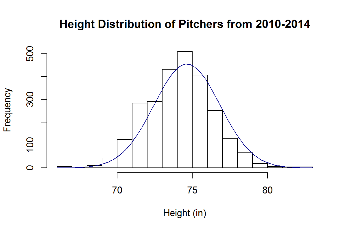
By this approximation, the chance of randomly selecting a pitcher of the last 5 years who is shorter than 5’11’’ is about 5%.

Are short pitchers really destined to fail? We’ve all been told that it’s better to be taller if you pitch. But is this true? Let’s consider short pitchers to be 5’11’’ or under and examine their effectiveness and distribution in comparison to taller pitchers, who we’ll consider to be 6 feet or taller.

The top ten best pitching seasons for shorter pitchers of the last 5 years are:

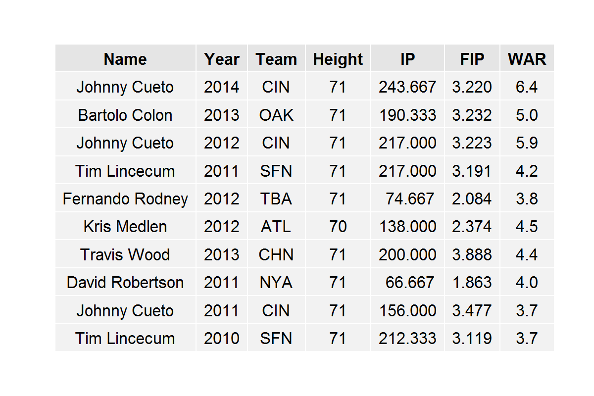
We notice that Tim Lincecum appears on this list twice and Johnny Cueto appears on it three times. All of these pitchers are 5’11’’ with the exception of Kris Medlen, who is 5’10’’. So, we see that successful pitching seasons by short pitchers don’t come completely out of the blue. Short pitchers can be successful and can dominate batters, most of whom are much taller, as Cueto did last year and in 2012.

In fact, short pitchers aren’t all that rare to come by, although they’re considerably rarer than taller pitchers. In the last 5 years, there have been 23 instances of short starting pitchers throwing at least 150 innings. In comparison, there have been 402 instances of this type for taller starting pitchers.

Shorter pitchers are generally relegated to the bullpen; there have been 95 instances in the last 5 years of full-time short relief pitchers and 968 instances of full-time taller relief pitchers.

We can see the average WAR breakdowns for all of these pools of players in the following table, along with P-Values for a two-sided t-test comparing the short relievers against the tall relievers and the short starters against the tall starters:

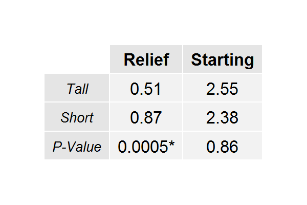
What the 0.0005 is telling us, here, is that we would observe these results by chance alone with probability 0.0005. Thus, there is actually a significant difference in the mean WAR for short relievers and the mean WAR for tall relievers (obviously favoring short relievers). On the other hand, the difference between the starters is not significant. Either way, we have no evidence to suggest that shorter pitchers are any less effective than taller pitchers.

Are shorter pitchers undervalued in the baseball market? If so, to what extent? We can approach this by examining the WAR value of a pitcher relative to his salary in free agency. We can do this by comparing the height groups within relievers and starters (since relievers are generally valued differently than starters).

However, we find that in the last five years, there are only 4 instances of a starter 5’11’’ or shorter pitching for a team that acquired him via free agency; and all of them are Bartolo Colon seasons from 2011-2014.

Fortunately, there are more instances of this in relievers, which is what we’ll examine. We notice the distribution of WAR and relievers’ salaries in free agency:

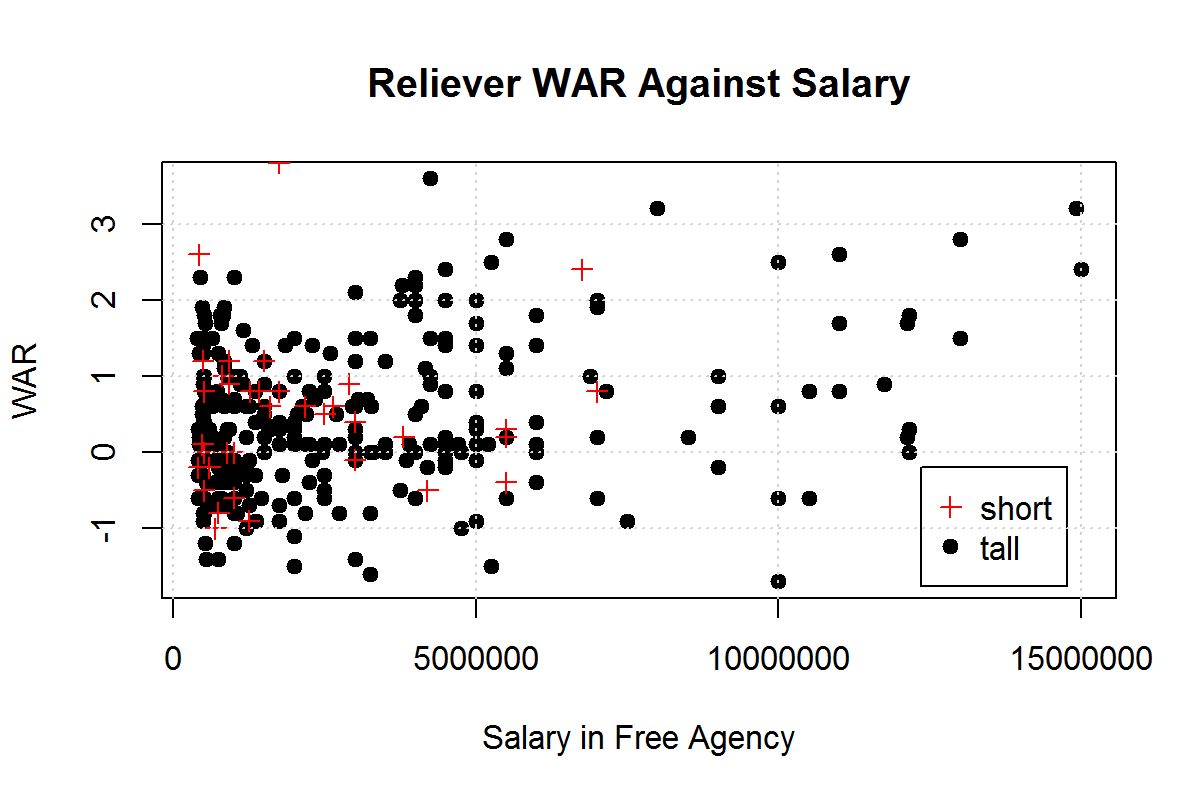
We see that short and tall relievers are clustered between -1 and 1 WAR and $1 million and $5 million dollars. However, we see several taller relievers past the $7.5 million mark with unremarkable WARs, which we don’t see for shorter relievers. From this, we would suspect that taller relievers are being overvalued while shorter relievers are being undervalued.

This is, in fact, the case: short relief pitchers are producing 2.33 WAR for every $10 million they earn in free agency while taller relievers are producing 1.36 WAR for every $10 million they earn. In comparing these values with a one-sided t-test, we acquire a P-Value of 0.0018, meaning these are results we would acquire by chance only .18% (a significant value) of the time. And so it goes, relievers under 6 feet are actually about 1.7 times as valuable as their taller counterparts.

Is there something inherently different about shorter pitchers that makes them less capable of pitching successfully in the big leagues? The evidence says no. In fact, it might be more worthwhile for General Managers to draft pitchers under 6 feet tall and reap the rewards.

Just because an athlete doesn’t tower over his opponents off the mound, doesn’t mean he can’t bring 55,000 dumbfounded Yankee fans to their feet on an unassuming September evening.

Let’s face it, people love the home run. It’s why players like Mark Reynolds can find jobs. These days, we aren’t surprised when we see a couple of home runs in one game. It wasn’t always like this, however. Home runs used to be a rarity among baseball events. In the early 20th century, it wasn’t uncommon for a player to lead his league in baseball by hitting 10-15 home runs. This brings me to the question: how has the home run actually changed? Not in terms of its frequency, but in terms of its value. More specifically, its value in runs. To approach a solution to this question without arduously parsing through hundreds of event files, we must find a way to mathematically frame the game of baseball in a way that encourages simplicity but doesn’t lose the most familiar parts of the game.

Markov Chains

The first batter of the game steps to the plate and sees no runners on base with none out. He pops up. The second batter steps to the plate and sees the immediate result of the last at bat: an out. The second batter walks. The third batter then sees the immediate result of the second batter’s at bat: a runner on first base. The stream of batters stepping to the plate and being placed into a state resulting from the previous batter’s at bat exemplifies the nature of a Markov Chain. When a batter steps into the batter’s box, his current state (whether it be an out situation, a base situation, or a base-out situation) is only dependent on the previous batter’s state. This is known as the Markov Property. Using this structure, we can simulate any baseball game we’d like. However, to keep our calculations simple, we should introduce some new rules.

The Rules of the Game

1. A batter can only attain a BB, HBP, 1B, 2B, 3B, or HR.
2. Outs only occur via a batter getting himself out.
3. Anything other than the events from 1) is assumed to be an out.
4. When a batter gets a hit, the runners on base advance by as many bases attained by the batter (e.g. a double with a runner on second will score the runner on second).

These are the rules of the game. There are no stolen bases, no scoring from second on a single, and no double plays. We have stripped the game down to only its essentials, while implementing certain changes for our own convenience. For our purposes, we don’t care about Mike Trout’s 33 stolen bases, only the fact that he mainly attains his bases through the events we allow.

The Out Chain

We assume that the probability of a batter getting a single at any point during a season is the number of singles he gets for the season divided by his plate appearances. We do this for the probabilities of all our desired events. By doing this, we can construct a simple Markov Chain where players step to the plate and find themselves batting with 0, 1, or 2 outs. We find that this chain is irreducible, meaning that each state (0, 1, or 2 outs) eventually leads to every other state. This, and the fact that we are dealing with a finite number of states, leads us to the existence of a probability distribution on our state space of outs. It so happens to be that when a batter starts his at bat, he does so with an equal probability of seeing 0, 1, or 2 outs, i.e. the probabilities of a batter seeing 0, 1, or 2 outs when he comes to the plate are all 1/3. The knowledge that outs are uniformly distributed over our game allows us to construct probabilities for a more complicated chain that should shed light on our original question.

The Base Chain

We now place our focus on the stream of batters who see a certain base situation when they step to the plate. The transitions of base situations are dependent on the out situation, as can be seen when a batter bats hits with 1 out versus 2 outs. Batting with 1 out, if the player makes another out, then the base situation stays the same for the subsequent batter. If he does this with 2 outs, however, then the inning is over and the base situation reverts to the state where no one is on base in the next inning. Fortunately, we know that the probability of a batter seeing any number of outs when he steps to the plate is 1/3. In a similar manner to the Out Chain, we find that every state in the Base Chain leads to every other state. The “runners on the corners” state eventually leads to the “bases loaded” state, which eventually leads to the “bases empty” state, and so on. Since there are finitely many base situations, we are led to a stationary probability distribution on the state space of base situations. That is to say, there is a probability associated with a runner stepping to the plate and seeing the bases empty, and another for seeing a runner on first, etc.

Results

Using this method, a player in our universe who stepped to the plate in 2013 saw the bases empty with an approximate probability of .467. That same batter saw the bases full with a probability of .103 and one runner on first with probability .210. If a team managed to load the bases, they’d find that they generally had to wait about 10 more plate appearances before they next loaded the bases. If they put runners on the corners, they generally had to wait 42 more plate appearances before they did so again. All of this leads us to some of our final conclusions. In the context of our rules, the expected number of runners on base in 2013 was .908, meaning that the expected value of a home run was 1.908 runs. This method generates home run values that are always between 1.8 and 2.2 runs. The following is a table of all of the expected home run values this method generates from the seasons of the last 25 years:

In the last 25 years, we predict that a home run had the greatest value in 1999, at 1.972 runs. This is a reflection of the heavily offensive environment of the season, when big bats such as Sammy Sosa, Mark McGwire, and Barry Bonds were getting on base at staggering rates. The following is a graph of all of the home run values the system predicts from 1884 through 2013:

We see that this system predicts home runs to have been of more value from around 1889 to 1902, when the home run hovers at around 2.00-2.15 runs. While most players of this generation weren’t hitting home runs, they were certainly getting on base often. In 1894, 38 players had on base percentages greater than or equal to .400, compared to 7 players in 2013. When on base percentages are higher, more people are on base, and this increases the expected value of the home run. Under our restrictions, however, the home run hasn’t been worth 2.00 runs since 1950 and these days it fluctuates between 1.90 and 1.93 runs. While these estimates are all under the umbrella of rules and assumptions, this framework allows us to more easily generalize the game of baseball while preserving its most important aspects. It’s this framework that gives us the power of estimating that, while Chris Davis‘ 53 home runs were probably worth 101 runs in 2013, they may have been worth 114 in 1894.