Classifying MLB Hit Outcomes

The exit velocity is the speed of the ball off of the bat, and the launch angle is the vertical angle off the bat (high values are popups, near-zero values are horizontal, negative values are into the ground). When these started becoming more popular, I found myself thinking quite often, “how do I know if this is good or not?” With exit velocity, it’s fairly easy to conceptualize, but things are less transparent for launch angle. This led me to try plotting these two variables using hit outcome as a figure of merit. The shown chart uses data from the 2018 season.

This plot held some interesting trends:

• A “singles band” stretching from roughly 45 degrees at 65 mph to -10 degrees beyond 100 mph. The former represents a bloop single while the latter is a grounder that shoots past infielders, and this band as a whole encapsulates everything in between.
• A considerable amount of stochastic singles at low launch speed. These can correspond to things like bunts against the shifts, infield hits, etc.
• A pocket for doubles with hard-hit balls (over ~85 mph), generally hit slightly above the horizontal, making it to the deep parts of the outfield.
• A well-defined home run pocket for hard-hit between 12-50 degrees.

A couple years after making this plot, I was thinking about where I could employ clustering models, and it jumped back to mind. Over the last few months, I’ve worked extensively on modeling this data.

Model Selection

While I approached this problem with clustering in mind, it’s always good to investigate other possible models. For this, I considered k-Nearest Neighbors (kNN) clustering, a Support Vector Classifier (SVC), and a Gradient Boosted Decision Tree (gBDT).

The previous plot looks at launch angle and exit velocity, but this neglects the third spatial dimension. In order to do this, I also included spray angle into the model, which captures horizontal location on the field, then I trained and evaluated each model to see which is most accurate. Click to enlarge:

Out of those evaluated, it turns out that tree-based methods perform the best out-of-box (77% accurate), so I chose that as the model of choice. A more extensive discussion of my model selection process can be found here.

Extending this model

In developing this model, I wanted to approach it as I would if I were a team: using parameters that are known in advance so I could use this model for player evaluation. The two most relevant parameters I looked at were player speed and differences in parks.

Player speeds were scraped from Baseball Savant. Since I’m evaluating on 2018 data, 2017 sprint speeds were assumed to be known and used in the model. For 2018 rookies, the mean sprint speed was imputed. By itself, adding sprint speed only marginally increased the accuracy of this model, but it did provide some improvement for accurately discerning extra-base hits, where speed can be very important.

To account for differences in parks, FanGraphs maintains park factor values to parameterize which outcomes are more likely in various parks. At the most granular level, they’re split by park type and handedness. When adding to the model, I consider the handedness of the player I’m evaluating and add all of the associated values. I again used 2017 park factor values (assuming they were known). These considerably helped the model, particularly discriminating home runs and doubles, improving the accuracy of both.

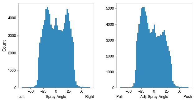
Last, inspired by a post about  fly ball carry on Alan Nathan’s blog, I replaced the absolute spray angle with an adjusted spray angle. Adjusted spray angle just flips the sign (from positive to negative, or vice-versa) for left-handed batters. By doing so, the information shifts from a sheer horizontal coordinate to a push-vs.-pull metric. Including this in the model rather than true spray angle helps it quite a bit, especially with quantifying home runs.

Additionally, I did a hyperparameter sweep of the model, adjusting parameters of the model itself. I found the optimum depth of the decision trees (think of a flowchart, splitting data more and more as it gets deeper) and learning rate (how much it adjusts to focus on previously misclassified data), which helped the model with singles and outs. Ultimately, a depth of 5 and a learning rate of 0.3 were used.

A full look at adding these parameters to the model and the hyperparameter optimization can be found in this blog post. The final model arrived at an accuracy of 79.14%.

Applying the Model

A common stat to evaluate offensive production is Weighted On Base Average (wOBA), which tries to encapsulate the idea that different offensive actions are worth different values and weights them proportionally to the observed “run value” of that action. The weights are derived from data, using a method known as linear weights.

The problem with wOBA is that it is calculated based on outcomes, but there’s a level of uncertainty in those outcomes – variance due to things like weather or defense. As a result, wOBA provides a good description of things that have happened, but not necessarily underlying skill. By focusing on wOBA, we do what Annie Duke calls “resulting” in her book Thinking in Bets – fixating solely on the outcome, neglecting the quality of inputs.

This is the perfect opportunity to utilize the model – the output assigns a probability for each hit type for balls hit in play. When describing accuracy in previous sections, the most probable outcome was compared to the true outcome, but it gives us the likelihood for all outcomes. For example, it might say a line drive has a 30% chance of an out, 40% chance of a single, 20% chance of a double, 10% chance at a triple, and isn’t hit hard enough for a homer (0% chance).

We can put these likelihoods into the wOBA calculation to get a value based on the probability the model assigns possible outcomes rather than only the result. To do so, the counts of each hit type in the wOBA calculation are replaced by the sum of probabilities for the respective hit type.

You might be thinking this sounds very familiar, and that’s because this is similar to what xwOBA is. Expected Weighted On-Base Average (xwOBA) does this calculation but has a different approach. For their model, line drives and fly balls are modeled with a k-Nearest Neighbors model using only exit velocity and launch angle, while soft hits are modeled with Generalized Additive Models (GAM) that also use sprint speed. To highlight some differences:

• Their model at no point uses spray angle, however my work showed spray angle helps accuracy significantly, and adjusted spray angle even more so.
• My model uses sprint speed everywhere. Speed is more important for infield events, so directly encoding like MLB’s model is almost certainly more helpful in those events, but I show it also helps with the accuracy of doubles, which almost entirely fall into the domain where MLB’s approach would not include speed.

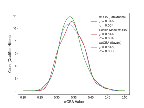
In order to put my model-based wOBA on the same scale as true wOBA and xwOBA, I scaled the mean and standard deviation of the distribution to that of true wOBA:

Now that they are comparable, I looked at how players are affected most, beginning with 2019 qualified hitters. Here’s a look at at model-based wOBA vs. true wOBA:

A full interactive version of this plot is available in this post. The grey line shown represents where wOBA predicted by the model matches true wOBA (y=x). Players above that line have a better model-based wOBA, and players under that line have a better true wOBA.

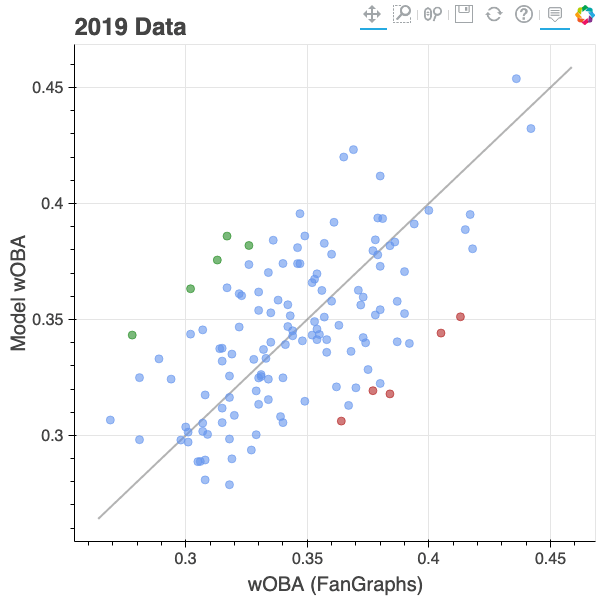
For those players above the line, the model believes that they have been unlucky in their outcomes and have disproportionately worse true outcomes with respect to wOBA, based on the hit kinematics, player speed, and park factors. The five players with the biggest difference between model-based and true wOBA are shown in green. Left to right they are: Mallex Smith, Rougned Odor, Willy Adames, Dansby Swanson, and Dexter Fowler. The high point on the far right above the line is Mike Trout – even with a true wOBA of 0.436, the model believes he was unlucky!

By contrast, the players the model thinks have gotten the most lucky in their outcomes are shown in red. Left to right: Yuli Gurriel, Rafael Devers, Jeff McNeil, Ketel Marte, and Anthony Rendon.

Reflection

In Scott Page’s The Model Thinker, he outlines seven possible uses for models under the acronym REDCAPE: Reason, Explain, Design, Communicate, Act, Predict, Explore. This is a machine-learning model, which are notoriously good at prediction at the cost of interpretability. Through these predictions, it can suggest acting. While the opacity of machine learning hurts interpretability, the development of has served to help explain as well.

Prediction

This model can be used to predict hit outcomes using just hit kinematics, player speed, and factors of the park you expect to be playing in. Because of this, it can be used for prediction in several regimes. However, it’s important to not make out-of-sample predictions, using the model somewhere it isn’t trained to. This model was trained on MLB data, so the domain of applicability is only for MLB-like scenarios. Due to differences in pitching skill, it won’t translate one-to-one to minor league data.

Where there is a clear value to prediction from this model would be situations in which starters practice against batters. In that case, it doesn’t matter the level of the batters, so long as the pitches they’re seeing are MLB-like. If there’s no defense on the field, it might not be clear how these practice hits would translate to real-world scenarios, but this model allows you to predict how the practice would translate to a real game. The scenario I can immediately think of is spring training, where minor leaguers are playing against MLB-caliber pitchers – this model would give you a more clear insight about what to expect from those minor leaguers in MLB game situations.

Acting

Elaborating from the previous prediction section, being able to understand hit outcomes from players who aren’t necessarily playing in MLB games is a powerful tool. It lets you better understand how to evaluate your players and motivate actions such as when to promote. Additionally, shown in the model-based wOBA application above, if wOBA is being used as a metric to evaluate player value, this can provide a more granular version of that, one that removes “resulting” from the equation and filters in some alternative outcome possibilities for the same hits. This would be very useful when doing things like evaluating trades if you know a player has been particularly unlucky recently and that the model predicts a higher wOBA than the true value.

Explaining

I have had been several interesting insights while developing this model, so I’ll wrap up with a few:

• Triples are tough to predict. Like, really tough. — This is an obvious statement in passing, but it wasn’t until fighting with this model to get any reasonable triple accuracy that I saw just how dire the situation was. They require the perfect coalescing of correct stadium, quick batter, slow fielder, and a solid hit, which make them incredibly unpredictable.
• Hit kinematics get you most of the way there in predicting the outcome of a hit — Beyond exit velocity, launch angle, and spray angle, further variables provided some improvements in accuracy, but nothing near the gain achieved by the initial three. This is important when considering things like the value of sprint speed — from an offensive perspective, it’s far secondary to a quality hit.
• Focusing on true outcomes loses understanding of underlying skill by neglecting the quality of inputs — In a high statistics regime, such as looking at all hits, there’s going to be many cases where less likely outcomes ended up being the true result; even a 5% probable event sounds low, but it still has a 1/20 opportunity of happening, which would occur a couple of times every game. Looking at possible outcomes rather than realized outcomes provides a better understanding of underlying talent.

I also encountered some model building insights that aren’t necessarily insights into the game itself, but they are still useful to keep in mind, especially for those building models:

• Smart features are just as useful as smart models — Taking a step back and using informative features is a great way to make sure your model is doing the best it can. for example, switching from absolute to adjusted spray angle provided a good improvement in accuracy.
• Simple questions can lead to useful projects — I made the launch angle vs. launch speed plot quite some time ago just because I was curious about how to interpret those parameters. That plot just sat in my head until I was thinking about projects I could use clustering on, which inspired this project.
• Sometimes your gut model isn’t the right one — I approached this problem thinking it’d be a neat way to employ k-Nearest Neighbors clustering. However, one of the first things I discovered is that tree-based methods do better than k-NN — keeping an open mind to alternative models is good, test as many as you can.

Hopefully you enjoyed this dive into model building and application. For a deeper look as well as links to code, be sure to check out my corresponding blog posts:

• Part 1: Model Selection
• Part 2: Optimization
• Part 3: Re-sampling Methods
• Part 4: Application and Reflection