Analyzing Underlying Factors Impacting Tickets Sold for Major League Baseball Games

I. Introduction

In 2017, Major League Baseball exceeded 10 billion dollars in total revenue for the first time. Ticket sales were a major component, making up 29.84 percent of this revenue (Statista.com). Due to the fact that fans continue to spend money once inside the stadium, 29.84 percent is merely a lower bound on revenue from ticket sales. For example, the average 2017 ticket price was 31 dollars; however, once inside the stadium, fans spent an average of 16 additional dollars on food (Statista.com).

II. Data

The data for this project are in an unbalanced panel format and contain 60,705 observations from 35 teams spanning from 1992 to 2017. Other than the 2017 season data, which I collected myself from baseballreference.com, the data from 1990 to 2016 were scraped from baseballreference.com by Troy Hepper, a consultant at Morgan Franklin Consulting, and shared on his github.com page.

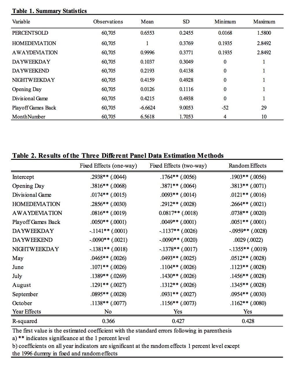
Descriptive statistics of my game by game data are displayed in Table 1. The dependent variable is the percentage of tickets sold relative to a stadium’s capacity (PERCENTSOLD). PERCENTSOLD ranges drastically from a little bit under 2 percent to over 150 percent with a mean of around 66 percent. PERCENTSOLD is sometimes greater than 1 because for certain important games ticket sales exceed stadium capacity; however, only 76 out of 60,705 observations exceed 110 percent and these outliers have almost no effect on the estimated coefficients in the models.

The explanatory variables in this model are designed to control for the time effects of when a baseball game was played, the quality of the home team, and the quality of the opponent. To control for the time that a game was played, indicators for the month and year are included in the model. To control for day of the week and whether or not the game was played at night or during the day, four dummy variables were created indicating whether or not a game was a night game during the week (NIGHTWEEKDAY), a day game during the week (DAYWEEKDAY), a night game during the weekend (NIGHTWEEKEND), or a day game during the weekend (DAYWEEKEND). Due to the immense popularity of the first game of the season, an indicator variable for Opening Day is also used.

The quality of the home team is assessed using both information on payroll and playoff chances. Better teams have better players and since players are paid based on skill and production, better teams consistently have higher payrolls. The payroll variable created here is the percentage deviation from league average payroll (HOMEDEVIATION). The minimum percentage deviation is a little under 20 percent of the league average while the maximum is over 280 percent of the league average. A standard deviation of a little under 40 percentage points shows the consistent variability of team payroll throughout the data. The playoff chances of a team are weighted by the number of games back or up they are on the guaranteed divisional playoff spot.

The quality of the visiting team is assessed using information on payroll and the opponent’s relationship with the home team. Fans want to come to the park to see good teams play so more attractive visiting teams will consistently have higher payrolls. The visiting team’s payroll variable (AWAYDEVIATION) is constructed the same way as the home team’s payroll discussed above. Because fans want to see their teams make the playoffs and the best way to do this is by beating the teams in your division, an indicator variable to assess the draw of a divisional game is used as well.

III. Regression Specification and Results

To better understand the relationship between the explanatory variables and the long-run demand for tickets, the data were analyzed using three panel data estimation techniques: one-way fixed effects, two-way fixed effects, and random effects models. For these data, it is clear that a fixed effects model is a better fit due to the fact that the unobserved metric of fan loyalty, which is constant over time, correlates very strongly with the two explanatory variables that control for payroll. The reason that fan loyalty is constant over time is that it is clear that for some teams, like the Chicago Cubs, the teams are deeply engrained in the culture of their cities and the fan bases remain loyal to these teams no matter what. On the other hand, for certain teams, like the Oakland Athletics, fan bases consistently disregard their teams and never become engaged. Because loyal fans spend more money and demand higher quality teams, owners of these teams must spend more on players. For this reason, payroll is correlated highly with the omitted variable, fan loyalty, making the use of a fixed effects essential for unbiased coefficient estimates.

The results of the three separate panel estimation techniques are recorded in Table 2; however, this paper will focus on the results of the following two-way fixed effects model:

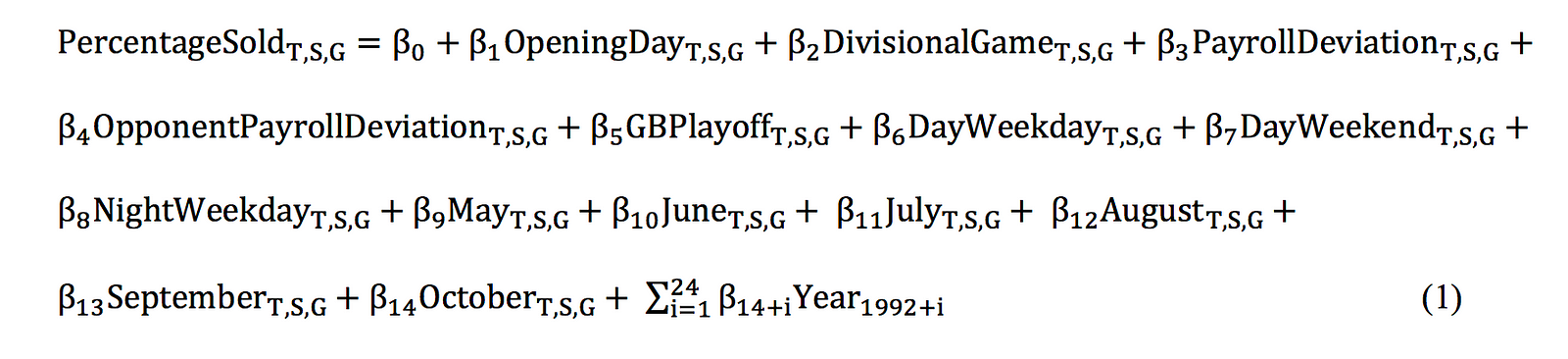
In this model, T represents the team, S represents the season, and G represents the gth home game for each season. An interesting conclusion is that except in the case of DAYWEEKEND, both the fixed and random effects estimation have the same sign and approximate magnitudes for each coefficient.

In the two-way fixed effects model, all variables except the time fixed effect for 1996 are significant at any standard level. The largest coefficient is that of the Opening Day dummy, which causes an estimated 38.7 percentage point increase in percentage of tickets sold. Interestingly, the year dummy variable shows an approximate 11 percentage point drop in PERCENTSOLD in 1995 in comparison to 1994. This drop is most likely due to the disdain towards baseball fans developed following the players’ strike of 1994. Another interesting league wide trend is the approximate 4 percentage point drop in PERCENTSOLD from 2007 to 2009 during the Great Recession. For the average sized stadium, this sized drop would result in a decrease of a little over 1,700 fans per game. According to statista.com, the average ticket price in 2009 was 26.6 dollars. Thus, the resulting setback of losing 1,700 fans paying 26.6 dollars per game over the course of 81 home games would be around 3.7 million dollars. According to the Hardball Times, league average revenue in 2007 was 171 million dollars so for the average team, a 3.7 million dollar drop in revenue in 2009 would result in around a two percentage point decline in revenue from ticket sales alone. This is economically significant for a profit maximizing firm like a baseball team.

Using April as the base case, the coefficients of all other month dummies are positive. This indicates that the first month of the season is the weakest month for maximizing PERCENTSOLD. Notably, July and August dominate the percentage of tickets sold with an estimated 13 to 14 percentage point increase in PERCENTSOLD in comparison to April. Economically, maximizing games played in July and August while scheduling off days during April would result in increased revenue; however, if three more games were scheduled in July and August, the increased number of fans paying the 2017 average price of 31 dollars per ticket would result in a little over 500,000 dollars in increased revenue, which is an economically insignificant increase of .2 percentage points.

The indicator variables designed to control for game time and game placement during the week also shed light on what type of games maximize PERCENTSOLD. In the model, NIGHTWEEKEND was left out and the coefficients of the other three dummies were negative. This tells us that weekend games played at night are the most popular. DAYWEEKEND seems to have the least effect decreasing PERCENTSOLD by around 1 percentage point, while NIGHTWEEKDAY has the most effect decreasing PERCENTSOLD by 14 percentage points.

The coefficient of HOMEDEVIATION can be interpreted as a 50 percentage point increase would result in a 14 percentage point increase in PERCENTSOLD. The other assessment of the home team, games back from the playoffs, predicts that for a five game lead on the division a team will see an approximate 2.5 percentage point increase in PERCENTSOLD while with a ten-game deficit a team will see a 5 percentage point decrease in PERCENTSOLD. This variable is particularly effective because on Opening Day everyone is 0 games back from the playoffs so it has no effect, but as the season continues and the games back variable becomes smaller or larger, its increased effect over the course of the season is naturally weighted in the model.

The coefficient AWAYDEVIATION has a smaller coefficient than HOMEDEVIATION, but is also positive and statistically significant. The effect of opponent is also shown in the divisional game dummy which tells us that if an opponent is in a team’s division, the percentage of tickets sold increases by a little under 1 percent. Although the divisional dummy is statistically significant, even if in 2017 the MLB had scheduled 40 more games against divisional opponents for each team, this change would have added under 500,000 dollars in revenue and increase total revenue by less than .2 percentage points, which is an economically insignificant change.

Overall, the data seem to tell the story that one would expect; however, it is always nice to attempt to quantify these relationships. For further information, the author can be contacted at marinojc@kenyon.edu.